Structured Independent Edge Model (SIEM)
Contents
4.6. Structured Independent Edge Model (SIEM)#
Next up, we’ll cover a statistical model for networks which generalizes the SBM from Section 4.2 a little differently than RDPG from Section 4.3. Sometimes in a network, there might particular pairs of nodes which, when those nodes are incident a particular edge, impart a different distribution for that edge. Let’s consider an example, which boils back to the example that we gave in Section 2. Imagine we have a network, where the \(n=100\) nodes are different areas of the brain. Each of these nodes are either in the left, or the right, side of the brain. An edge exists, or does not exist, if the two areas of the brain tend to be active together while a person iteracts with the world. A particular notion that scientists hypothesis is that, even though the left and right sides of the brain tend to have different functions, the nodes on the left and right sides still might tend to be active together, especially when it is the same region on both sides. For instance, even though the motor cortex (responsible for motion and conscious movement) in the left hemisphere has different jobs from the motor cortex in the right hemisphere, the jobs provided by each hemisphere tend to work in tandem, with the right motor cortex providing movement for the left side of the body, and the left motor cortex provides movement for the right side of the body. When someone is moving around, a lot of tasks will require them to use both sides of the body in tandem, so even though the two motor cortexes are doing different jobs, they still tend to be active together. This pattern, known as bilateral homotopy, tends might trickle down to many other nodes in the brain as well. Let’s turn this into a question: do bilateral node pairs have higher connectivity than non-bilateral node pairs?
So, how do you actually study this property? As we have learned in this chapter so far, we want statistical models which capture what we understand about the system. What you understand is that, perhaps, the edges between pairs of nodes which are bilaterally symmetric tend to be more likely than the edges between pairs of nodes which are not bilaterally symmetric. Based on what we know so far, you could reflect this using a \(SBM\) as follows: for every node, find its bilateral pair, and place them in their own group. If there are \(100\) nodes each of which has a bilateral pair, this would give you \(K=50\) communities (one for each pair of nodes), and consequently, a \(50 \times 50\) block probability matrix which has \(\frac{1}{2} \cdot 50 \cdot 49 = 1225\) probability parameters. However, our overarching question is not about this particular arrangement of the nodes: our statement is about node pairs overall, not about any particular pair of nodes. If we were to use this grouping of the nodes in the network, we would only know about paritcular pairs of nodes (a community-by-community approach), which is not what we want to do!
Instead, we will conceptualize this problem a little bit differently using the Structured Independent Edge Model (SIEM).
4.6.1. The Structured Independent Edge Model is parametrized by a Cluster-Assignment Matrix and a probability vector#
To describe the Structured Independent Edge Model (SIEM), we will return to our old coin flipping example.
4.6.1.1. The Cluster-Assignment Matrix#
The cluster assignment matrix \(Z\) is an \(n \times n\) matrix which assigns potential edges in the random network to clusters. What do we mean by this?
Remember that the adjacency matrix \(\mathbf A\) for a random network is also an \(n \times n\) matrix, where each entry \(\mathbf a_{ij}\) is a random variable which takes the value \(0\) or the value \(1\) with a particular probability. The cluster assignment matrix takes each of these \(n^2\) random variables, and uses a parameter \(z_{ij}\) to indicate which of \(K\) possible clusters this edge is part of. In the school example, for instance, the edges in the upper left and lower right are in cluster \(1\) (‘within-school’ edges), and the edges in the upper right and lower left are in cluster \(2\) (‘between-school’ edges). In the school example, \(K=2\).
4.6.1.2. The Probability vector#
the second parameter for the SIEM is a probability vector, \(\vec p\). If there are \(K\) edge clusters in the SIEM, then \(\vec p\) is a length-\(K\) vector. Each entry \(p_k\) indicates the probablity of an edge in the \(k^{th}\) cluster existing in the network. For example, \(p_1\) indicates the probability of an edge in the first edge cluster, \(p_2\) indicates the probability of an edge in the second edge cluster, so on and so-forth. In the school example, for instance, the probability \(p_1\) indicates the probability of a within-school edge, and the probability \(p_2\) indicates the probability of a between-school edge.
Like usual, we will formulate the SIEM using our old coin flip example. We begin by obtaining \(K\) coins, where the \(k^{th}\) coin has a chance of landing on heads of \(p_k\), and a chance of landing on tails of \(1 - p_k\). For each entry \(\mathbf a_{ij}\), we identify the corresponding cluster \(z_{ij}\) that this edge is in. Remember that \(z_{ij}\) takes one of \(K\) possible values. We flip the \(z_{ij}\) coin, and if it lands on heads (with probability \(p_{z_{ij}}\)), the edge exists, and if it lands on tails (with probability \(1 - p_{z_{ij}}\)) the edge does not exist.
If \(\mathbf A\) is an SIEM random network with \(n\) nodes, the cluster assignment matrix \(Z\), and the probability vector \(\vec p\), we say that \(\mathbf A\) is an \(SIEM_n(Z, \vec p)\) random network.
4.6.1.3. How do we simulate samples from an \(SIEM_n(Z, \vec p)\) random network?#
The procedure below will produce for us a network \(A\), which has nodes and edges, where the underlying random network \(\mathbf A\) is an \(SIEM_n(Z, \vec p)\) random network:
Simulating a sample from an \(SIEM_n(Z, \vec p)\) random network
Determine a cluster assignment matrix \(Z\) for each edge of the network. Each edge entry \(z_{ij}\) can take one of \(K\) possible values.
Determine a length-\(K\) probability vector for each of the \(K\) edge clusters.
For each of the \(K\) clusters, obtain \(K\) total weighted coins, where the \(k^{th}\) coin lands on heads with probability \(p_k\) and tails with probability \(1 - p_k\).
For each edge \((i, j)\):
Denote \(z_{ij}\) to be the cluster assignment of the potential edge between node \(i\) and node \(j\).
Flip the \(z_{ij}\) coin, and if it lands on heads, the corresponding entry in the adjacency matrix \(a_{ij}\) is \(1\). If it lands on tails, the coresponding entry in the adjacency matrix \(a_{ij}\) is \(0\).
The adjacency matrix we produce, \(A\), is a sample of an \(SIEM_n(Z, \vec p)\) random network.
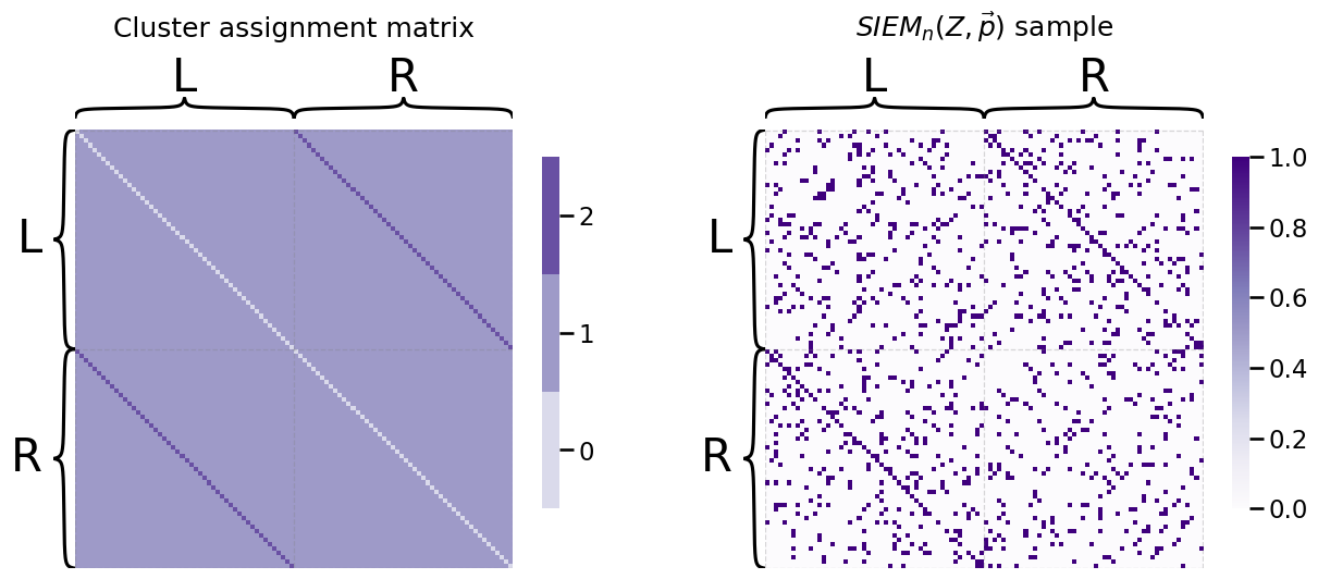
Let’s turn back to our network example we looked at. The first fifty nodes will be the areas in the left hemisphere of the brain, and the second fifty nodes will be the areas of the right hemisphere of the brain. The nodes will be sequentially ordered, so that the first node of the left is the first node of the right, so on and so forth, for all \(50\) pairs of nodes. The cluster assignment matrix looks like this:
from graphbook_code import siem, heatmap
import numpy as np

n = 100
Z = np.ones((n, n))
for i in range(0, int(n/2)):
    Z[int(i + n/2), i] = 2
    Z[i, int(i + n/2)] = 2
np.fill_diagonal(Z, 0)
Z = Z.astype(int)
labels = ["L" for i in range(0, int(n/2))] + ["R" for i in range(0, int(n/2))]
heatmap(Z, title="Cluster assignment matrix", inner_hier_labels=labels);
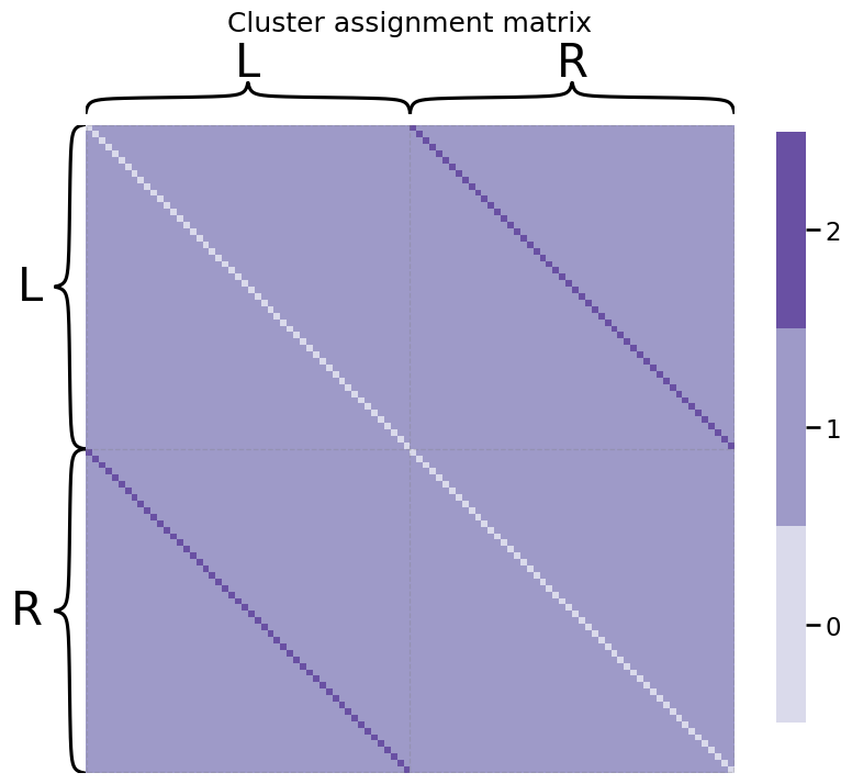
As we can see, there are several bands going across this matrix. We can see the white band is the diagonal entries. Since the networks we are dealing with are simple, they are undirected, so we do not need to worry about the diagonal entries.
In the off-diagonal entries, we can see another band. This band consists of the bilateral pairs of nodes; remember that the first node of the left hemisphere was the same functional area of the brain, but just in the other hemisphere. Hence, these edges are “assigned” to cluster \(2\).
The remaining off-diagonal entries are not bilateral pairs of nodes. These entries are assigned to cluster \(1\).
Next, we need a probability vector for the two clusters of off-diagonal entries. We will arbitrarily say that there is a \(0.8\) probability that an edge adjoining two bilateral pairs of nodes (cluster \(2\)) is connected, but a \(0.1\) probability that an edge adjoining two non-bilateral pairs of nodes (edge cluster \(1\)) is connected:
p = [0.1, 0.8]
A = siem(n, p, Z)
from matplotlib import pyplot as plt

fig, axs = plt.subplots(1, 2, figsize=(15, 6))
heatmap(Z, title="Cluster assignment matrix", inner_hier_labels=labels, ax=axs[0])
heatmap(A, title="$SIEM_n(Z, \\vec p)$ sample", inner_hier_labels=labels, ax=axs[1]);
4.6.2. Why do we care about the SIEM?#
If you recall from Section 4.3, we learned that for every \(SBM_n(\vec z, B)\) random network, there is a corresponding latent position matrix \(X\) such that the probability matrices of the \(SBM_n(\vec z, B)\) random network and an \(RDPG_n(X)\) random network are the same. In this sense, the RDPG random networks generalize the SBM random networks, in that all SBM random networks are RDPG random networks, but not all RDPG random networks are SBM random networks. We can find latent position matrices which produce networks which cannot be summarized with an SBM, such as the Section 4.3. The SIEM has a similar relationship with the SBM: all SBM random networks are SIEM random networks, but not all SIEM random networks are SBM random networks. If you want the gorey details of how this works, check out the block below. If not, you can skip on to the next paragraph.
All SBMs are SIEMs
What this means is that for any \(SBM_n(\vec z', B)\) random network, there is a corresponding \(Z\) and \(\vec p\) such that an \(SIEM_n(Z, \vec p)\) random network has the same probability matrix. We can see this pretty easily: if \(K\) was the number of communities of the SBM, we can define an SIEM to have a single edge cluster for each pair of communities. We can see this as follows:
Define the number of edge clusters: Edge cluster \(1\) consists of edges between nodes both in community \(1\), edge cluster \(2\) consists of edges between a node in community \(1\) and a node in community \(2\), so on and so forth up to edges between a node in community \(1\) and a node in community \(K\). Edge cluster \(K+1\) consists of edges between a node in community \(2\) and a node in community \(1\), and again we repeat this up to edge cluster \(2K\) which delineates edges between a node in community \(2\) and a node in community \(K\). We continue this procedure up to edge cluster \(K^2\) which is between two nodes in community \(K\). This gives us a map, where for each pair of communities \(l\) and \(l'\), we have an edge cluster \(k\) whch corresponds to this pair of communities.
Define the edge cluster matrix: Proceed edge-by-edge through the network looking at the community asignment vector \(\vec z'\). The edge cluster for an edge \((i, j)\) is the edge cluster we identified above between the communities for node \(i\) and node \(j\), \(z_i'\) and \(z_j'\) respectively.
Define the edge cluster probability vector: Let the probability vector \(\vec p\) be defined such that, iff the \(l\) and \(l'\) communities correspond to edge cluster \(k\), then \(p_k\) has the same value as \(b_{ll'}\) in the block matrix. This produces an \(SIEM_n(Z, \vec p)\) random network with the same probability matrix as an \(SBM_n(\vec z, B)\) random network.
For this reason, in later sections such as Section 6.2, we will develop statistical tools for the SIEM, but it is important to note that they apply equally well to an SBM random network. The statistical tools afforded to the SIEM will allow you to capture more general questions than just those you could ask with the SBM, in which you can look for differences between pairs of groups of edges, rather than just looking for differences between pairs of groups of nodes, since there can be complicated arrangements of edges which are not easily capturable with the SBM.