6.2. Testing for Differences between Groups of Edges

Let’s recall back to our school example. We have a network consisting of \(100\) students who attend one of two schools, with the first \(50\) students attending school one and the second \(50\) students attending school two. The nodes are students, and the edges are whether a pair of students attend the same school. What we want to know is whether there is a higher chance two students are friends if they go to the same school than if they go to two different schools. Since our hypothesis is about schools, we’ll assume we already know which school each individual goes to. Our network looks like this:

from graspologic.simulations import sbm
import numpy as np

# define the parameters for the SBM
ns = [50, 50]
n = np.array(ns).sum()
B = [[0.6, 0.4],[0.4, 0.6]]
zs = [1 for i in range(0, ns[0])] + [2 for i in range(0, ns[1])]

A = sbm(n=[50, 50], p=B, loops=False, directed=False)

from graphbook_code import draw_multiplot
import matplotlib.pyplot as plt

draw_multiplot(A, labels=zs, title="School Network Sample");

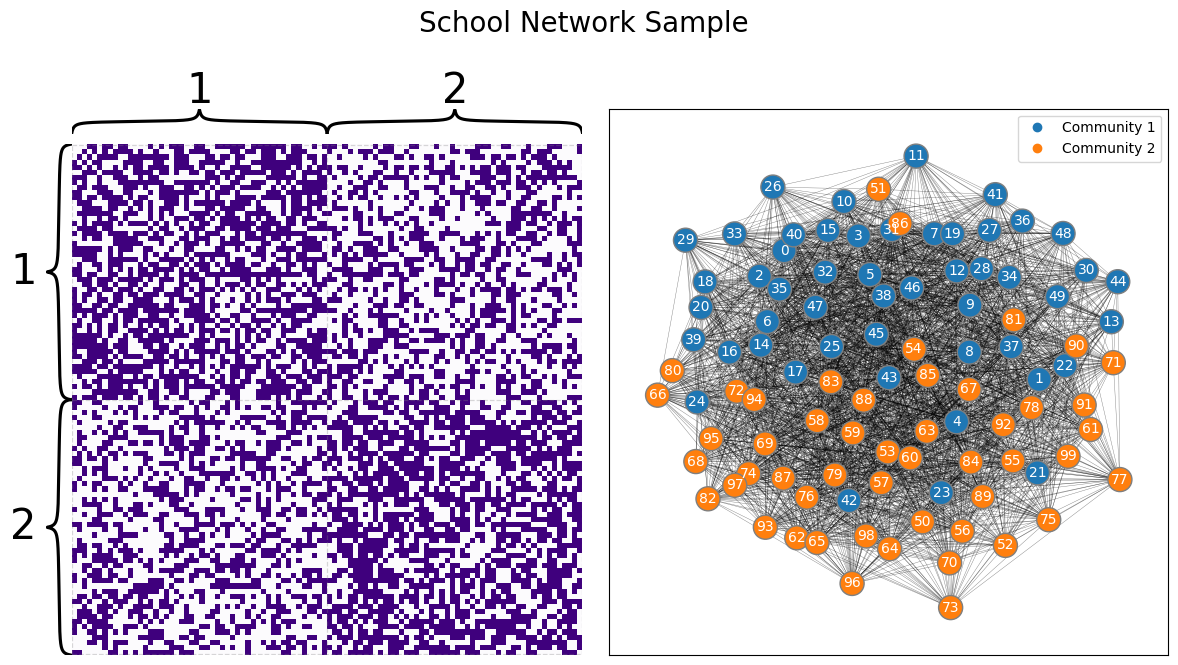
Looking at the network, it looks like, just maybe, our hypothesis could be true, and it’s possible that there is a higher chance that two students have a higher chance of being friends if they are both from the same school than if they go to different schools.

The true, but unknown, probability matrix looks something like this:

z = np.array([[1, 0] for i in range(0, ns[0])] + [[0, 1] for i in range(0, ns[1])])
P = z @ B @ z.T

from graphbook_code import heatmap, text

fig, ax = plt.subplots(1,1, figsize=(8, 6))
heatmap(P, vmin=0, vmax=1, ax=ax, title='True Probability Matrix, School Network')
text(x=.25, y=.75, label=B[0][0], color="white", ax=ax)
text(x=.75, y=.25, label=B[1][1], color="white", ax=ax)
text(x=.75, y=.75, label=B[1][0], color="black", ax=ax)
text(x=.25, y=.25, label=B[0][1], color="black", ax=ax)
fig;

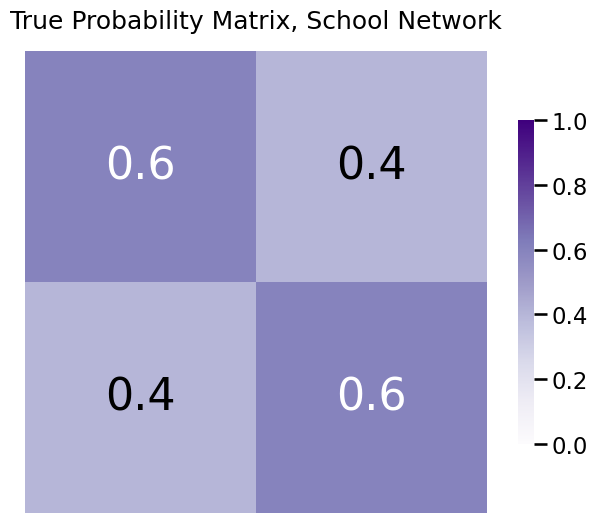
So, in actuality, it is the case that the true probabilities are higher if two students are from the same school than if they are from different schools. However, we don’t get to see this true probability matrix when we perform our analysis; we only see the sample.

How do we proceed?

Let’s think of how to better formulate this problem.

Everything we have done up until this point in the book treated nodes as the fundamental objects of interest for statistical modelling. We have communities of nodes, and clusters of latent positions corresponding to nodes which comprise these communities.

Well, everything except the model we will turn to here: the Structured Independent Edge Model (SIEM) from Section 4.6.

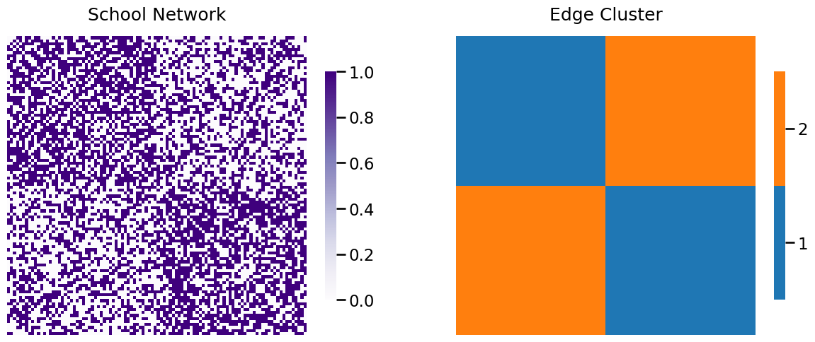
In the structured independent edge model, if you remember, we instead focuses on clusters of edges. Notice that the edges amongst students of school one are all in the upper left square of the adjacency matrix, and the edges amongst students of school two are all in the lower right square of the adjacency matrix. We will call these edges the “within-school” edges (Cluster \(1\)). The edges between students of school one and two are in the upper right and upper left squares of the adjacency matrix (Cluster \(2\)). In a picture, the edges are grouped as follows:

Z = np.zeros((n,n))

Z[0:50,0:50] = 1  # within-school edge
Z[0:50,50:100] = 2  # between-school edge
Z[50:100,50:100] = 1  # within-school edge
Z[50:100,0:50] = 2  # between-school edge

from graphbook_code import heatmap

fig, ax = plt.subplots(1,2,figsize=(15, 6))

heatmap(A, ax=ax[0], title='School Network')
heatmap(Z.astype(int), ax=ax[1], color="qualitative", n_colors=2, title="Edge Cluster");

6.2.1. Hypothesis testing

Remember that our question boiled down to whether the edges which are assigned to cluster \(1\) have a higher probability of existing than the edges of cluster \(2\). In other words, we hypothesize that the edges assigned to cluster \(1\) have a higher probability of existing than the edges of cluster \(2\). In terms of the probability vector, what we are saying is that we think that \(p_1 > p_2\). Obviously, we are wrong if \(p_1 \leq p_2\). This type of statistical question is known as a hypothesis test.

Hypothesis testing is an approach by which we formulate statistical questions and present approaches which, using the data, indicates how much the data supports or doess not support the statistical questions we asked (or, provide us with the ability to infer something). For this reason, hypothesis testing is often an essential component of statistical inference, which is the name given to the process of learning something from data using statistical models.

The way hypothesis testing works is we call one hypothesis a null hypothesis and the other an alternative hypothesis.

The null hypothesis is the hypothesis where, if true, indicates that we were wrong about what how we thought the system behaved. In our example data, the null hypothesis is that \(p_1 \leq p_2\). We typically would write this out notationally as \(H_0: p_1 \leq p_2\). The capital \(H\) is used to denote that this is a hypothesis, and the little “\(0\)” is just to indicate “null”.

The alternative hypothesis is the hypothesis where, if true, indicates that we werer correct about how we thought the system behaved. In our example, the alternative hypothesis is that \(p_1 > p_2\), which we write out as \(H_A: p_1 > p_2\). Here, the subscript \(A\) denotes that this is the alternative hypothesis.

When describing our hypothesis, we say that we are testing \(H_A: p_1 > p_2\) against \(H_0: p_1 \leq p_2\). This is because a hypothesis test must specifically delineate the possible situations in which we are right (the alternative \(H_A\)) and when we are wrong (the null \(H_0\)). We perform statisical inference by looking at how well the data we are presented with reflects the null hypothesis. This means that either the data looks like what we would expect under the null hypothesis (and the \(p\)-value is large) or the data does not look like what we would expect under the null hypothesis (and the \(p\)-value is small).

If you are unfamiliar or need a refresher on hypothesis testing, please see the appendix section hypothesis testing with coin flips in Section 13.1. There, we will cover some basics such as the details of a hypothesis test, the intuition of a one-sided hypothesis test, and how hypothesis tests relate back to statistical models, which will be valuable for you as you come into contact with hypothesis tests more and more in the applications of the material you are learning here.

6.2.1.1. Caveats of hypothesis testing

Before we jump in, we want to emphasize a few misconceptions about hypothesis testing that permeate many aspects of science.

The first misconception is that true or false, in the context of a hypothesis test, don’t really mean true or false in the traditional sense. A hypothesis test is tied directly to the statistical model used to describe the data: a hypothesis can be true or false with respect to a statistical model which is assumed to be true, but hypotheses on the basis of real data can either be supported by the data or unsupported by the data. This is because the statistical model which is used to describe the real data is, almost always, never actually true.

Second, hypothesis tests make statements about underlying parameters of the assumed statistical model on the basis of the data that you obtain. This is why, in the example that we gave above about coin flipping, the probabilities are \(p_1\) and \(p_2\) (the actual probabilities that the coins land on heads), and not \(\hat p_1\) nor \(\hat p_2\) (the estimated probabilities that the coins land on heads, which we would estimate from our sample). Even when the statistical model is true (which, as we stated, is never the case), analysis of the sample is also almost never going to give you the true underlying parameters of the data sample. This reinforces that, even if the statistical model were true (which it isn’t), you still can only conclude that a hypothesis is supported or unsupported by the data.

Finally, we get to the most pervasive caveat of hypothesis testing. Statistical hypothesis testing makes statements about the null hypothesis being either supported or unsupported by the data. There are two outcomes for a typical hypothesis test. In the first outcome, the null hypothesis is unsupported by the data, and the language you use is that you “reject the null hypothesis in favor of the alternative hypothesis.” The possible second outcome is that you “cannot reject the null hypothesis.” Note that this outcome makes no statement about the null hypothesis being supported by the data: you do not accept the null hypothesis when you conduct a hypothesis test, you just don’t have enough evidence to reject it.

Armed with these caveats, let’s rotate back to hypothesis testing.

6.2.1.1.1. Two-sample hypothesis testing with coins

Let’s say you are playing a gambling game. A gambler proposes a game to you in which he has two coins, and tells you that the first coin is for you and the second coin is for him. You gamble one dollar, and if your coin comes up heads but his comes up tails, you get your dollar plus an additional dollar. If both coins land on heads or tails, you get your dollar back. If his coin comes up heads but your coin comes up tails, you lose your dollar. You get to see the gambler flip each coin ten times before determining whether you want to play. Your coin lands on heads seven times, and his coin lands on heads three times. If your coin has a higher probability of landing on heads than his coin, you should play the game. Will you gamble?

To formalize this situation, we’ll use similar notation to before. We’ll call \(p_1\) the probability that your coin lands on heads, and \(p_2\) the probability that his coin lands on heads. Our alternative hypothesis here is \(H_A: p_1 \neq p_2\), against the null hypothesis \(H_0: p_1 = p_2\). A two-sample test is a test which is performed when we have two random samples, and we want to investigate whether there is a difference between the two random samples. Specifically here, we have the outcomes of coin flips from each of the two coins, and we want to determine whether your coin actually has a higher probability of landing on heads than his coin. Intuitionally, the idea is that even if your coin did not have a higher probability of landing on heads than his coin, there is still some probability that if we flipped each coin ten times, we would get more heads with the second coin. We see that our estimates of the probabilities are \(hat p_1 = \frac{7}{10} = 0.7\) and \(\hat p_2 = \frac{3}{10} = 0.3\) respectively.

When we have two samples of data whose outcomes boil down to ones and zeros (or, heads and tails), it turns out that the intuition gets more complex pretty quickly. For this reason, we won’t explain the two-sample test for binary data in quite as much depth as we did with the example we provided in the appendix Section 13.1 (the one-sample test), but much of the same intuition holds. Again, we seek to compute a \(p\)-value which tells us the chances of observing that \(\hat p_1 = 0.7\) and \(\hat p_2 = 0.1\) if \(p_1\) weren’t actually greater than \(p_2\). In this case, the appropriate statistical test is known as Fisher’s Exact Test [1] [2], which we can implement using scipy. The inputs for Fisher’s exact test is a contingency table of the results:

	First coin	Second coin
Landed on heads	7	3
Landed on tails	3	7

from scipy.stats import fisher_exact

table = [[7,3], [3,7]]
test_statistic, pval = fisher_exact(table)
print("p-value: {:.3f}".format(pval))

p-value: 0.179

This means that, there is about an \(17.9\%\) chance that the two coins have the same probability of landing on heads, as the \(p\)-value is \(0.179\). Fisher’s exact test is a two-sided test, which means that to determine which probability exceeds which, we need to do some more work. If you were to use \(\alpha=0.05\) as your decision threshold, you might not want to commit all your money just yet. With \(\alpha=0.05\), this would not be enough evidence to reject the null hypothesis in favor of the alternative hypothesis, and you might not want to play the game.

Next, we’ll see how this strategy of coin flipping applies to the SIEM.

6.2.1.2. Hypothesis Testing using the SIEM

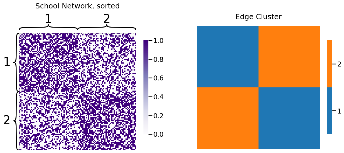
To shift back to our network, we had the following network sample and edge cluster matrix:

from graphbook_code import heatmap, cmaps

fig, ax = plt.subplots(1,2,figsize=(15, 6))

heatmap(A, ax=ax[0], inner_hier_labels=zs, title='School Network, sorted')
heatmap(Z.astype(int), ax=ax[1], color="qualitative", title="Edge Cluster");

The probability vector for the SIEM is estimated very similar to how we used maximum likelihood estimation for the SBM, in that we just take the fraction of edges which exist in the network for each edge cluster:

p = [np.sum(A[Z == i])/np.size(A[Z == i]) for i in [1, 2]]
[print("Probability for cluster {}, p{}: {:.3f}".format(i, i, p[i - 1])) for i in [1, 2]];

Probability for cluster 1, p1: 0.595
Probability for cluster 2, p2: 0.416

These estimates are pretty different, but the core question we want to answer is, how confident are we that this discrepancy between the estimated probabilities is not due to random chance?

It turns out that this question is effectively the same question as we asked for the coin flips. Specifically, we want to formulate the hypothesis test with \(H_0: p_1 \leq p_2\) against \(H_A: p_1 > p_2\). We proceed with exactly the same framework as we used for the coin tosses. We again construct a contingency table, with the following table cells:

	Cluster 1, the within-school edges	Cluster 2, the between-school edges
Number of edges	\(a\)	\(b\)
Number of non-edges	\(c\)	\(d\)

The entry \(a\) is the total number of edges in the first cluster, and \(b\) is the total number of edge in the second cluster. The entry \(c\) is the total number of possible edges in cluster one which do not exist (the number of adjacencies in cluster one with an adjacency of zero), and the entry \(d\) is the total number of possible edges in the second cluster which do not exist (the number of adjacencies in cluster two with a value of zero). We can fill in the entries of this table using some basic numpy functions. Note that since this network is undirected and loopless, we want to look only at the edges which are in the upper triangle of the adjacency martix, and exclude the diagonal:

# get the indices of the upper triangle of A
upper_tri_idx = np.triu_indices(A.shape[0], k=1)
# create a boolean array that is nxn
upper_tri_mask = np.zeros(A.shape, dtype=bool)
# set indices which correspond to the upper triangle to True
upper_tri_mask[upper_tri_idx] = True

table = [[(A[(Z == 1) & upper_tri_mask] == 1).sum(), np.sum(A[(Z == 2) & upper_tri_mask] == 1)],
         [(A[(Z == 1) & upper_tri_mask] == 0).sum(), np.sum(A[(Z == 2) & upper_tri_mask] == 0)]]

from graphbook_code import cmaps
import seaborn as sns

fig, ax = plt.subplots(1,1,figsize=(8, 6))
sns.heatmap(np.array(table, dtype=int), ax=ax, square=True, cmap=cmaps["sequential"],
            annot=True, fmt="d", vmin=0, cbar_kws={"label": "Count"})
ax.set_xticks([0.5, 1.5])
ax.set_xticklabels(["Cluster 1", "Cluster 2"])
ax.set_yticks([0.5, 1.5])
ax.set_yticklabels(["Number of edges", "Number of non-edges"], rotation=0)
ax.set_title("Contingency Table, School Network");

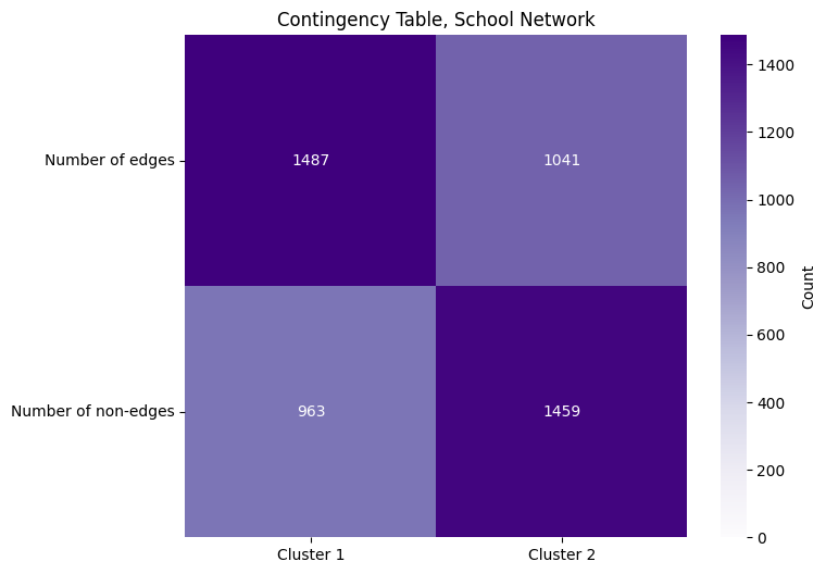
We again use Fisher’s exact test to test our hypothesis:

test_statistic, pval = fisher_exact(table)
print("p-value: {:.3f}".format(pval))

p-value: 0.000

And we end up with a \(p\)-value that is approximately zero. With our decision threshold still at \(\alpha = 0.05\), since the \(p\)-value is less than \(\alpha\), we have evidence to support that we should reject the null hypothesis. So, after a lot of build up spanning numerous sections, we have shown that the probability of two individuals being friends if they attend the same school is higher than the probability of two students being friends if they go to different schoools. Pretty exciting, huh?

6.2.2. References

In the appendix, we also go through the two-sample test for network edges in weighted network in Section 13.1.2. Check it out for more details! Most of the results that we presented in this section can be attributed to several areas of research, including [1] and [4].

1

R. A. Fisher. On the Interpretation of χ 2 from Contingency Tables, and the Calculation of P. Zenodo, January 1922. doi:10.2307/2340521.

2

R. A. Fisher. Statistical Methods for Research Workers. In Breakthroughs in Statistics, pages 66–70. Springer, New York, NY, New York, NY, USA, 1992. doi:10.1007/978-1-4612-4380-9_6.

3

Benjamin D. Pedigo, Mike Powell, Eric W. Bridgeford, Michael Winding, Carey E. Priebe, and Joshua T. Vogelstein. Generative network modeling reveals quantitative definitions of bilateral symmetry exhibited by a whole insect brain connectome. bioRxiv, pages 2022.11.28.518219, November 2022. URL: https://doi.org/10.1101/2022.11.28.518219, arXiv:2022.11.28.518219.

4

Jaewon Chung, Eric Bridgeford, Jesús Arroyo, Benjamin D. Pedigo, Ali Saad-Eldin, Vivek Gopalakrishnan, Liang Xiang, Carey E. Priebe, and Joshua T. Vogelstein. Statistical Connectomics. Annu. Rev. Stat. Appl., 8(1):463–492, March 2021. doi:10.1146/annurev-statistics-042720-023234.