3.1. Matrix Representations Of Networks

When we work with networks, we need a way to represent them mathematically and in our code. A network itself lives in network space, which is just the set of all possible networks. Network space is kind of abstract and inconvenient if we want to use traditional mathematics, so we’d generally like to represent networks with groups of numbers to make everything more concrete.

More specifically, we would often like to represent networks with matrices. In addition to being computationally convenient, using matrices to represent networks lets us bring in a surprising amount of tools from linear algebra and statistics. Programmatically, using matrices also lets us use common Python tools for array manipulation like numpy.

A common matrix representation of a network is called the Adjacency Matrix, and we’ll learn about that first.

3.1.1. An Adjacency Matrix

Throughout this book, the beating heart of matrix representations of networks that we will see is the adjacency matrix [1]. The idea is pretty straightforward: Let’s say you have a network with \(n\) nodes. You give each node an index – usually some value between 0 and n – and then you create an \(n \times n\) matrix. If there is an edge between node \(i\) and node \(j\), you fill the \((i, j)_{th}\) value of the matrix with an entry, usually \(1\) if your network has unweighted edges. In the case of undirected networks, you end up with a symmetric matrix with full of 1’s and 0’s, which completely represents the topology of your network.

Let’s see this in action. We’ll make a network with only three nodes, since that’s small and easy to understand, and then we’ll show what it looks like as an adjacency matrix.

import numpy as np
import networkx as nx

G = nx.DiGraph()
G.add_node("0", pos=(1,1))
G.add_node("1", pos=(4,4))
G.add_node("2", pos=(4,2))
G.add_edge("0", "1")
G.add_edge("1", "0")
G.add_edge("0", "2")
G.add_edge("2", "0")

pos = {'0': (0, 0), '1': (1, 0), '2': (.5, .5)}

nx.draw_networkx(G, with_labels=True, node_color="tab:purple", pos=pos,
                font_size=10, font_color="whitesmoke", arrows=False, edge_color="black",
                width=1)
A = np.asarray(nx.to_numpy_matrix(G))

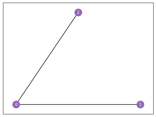
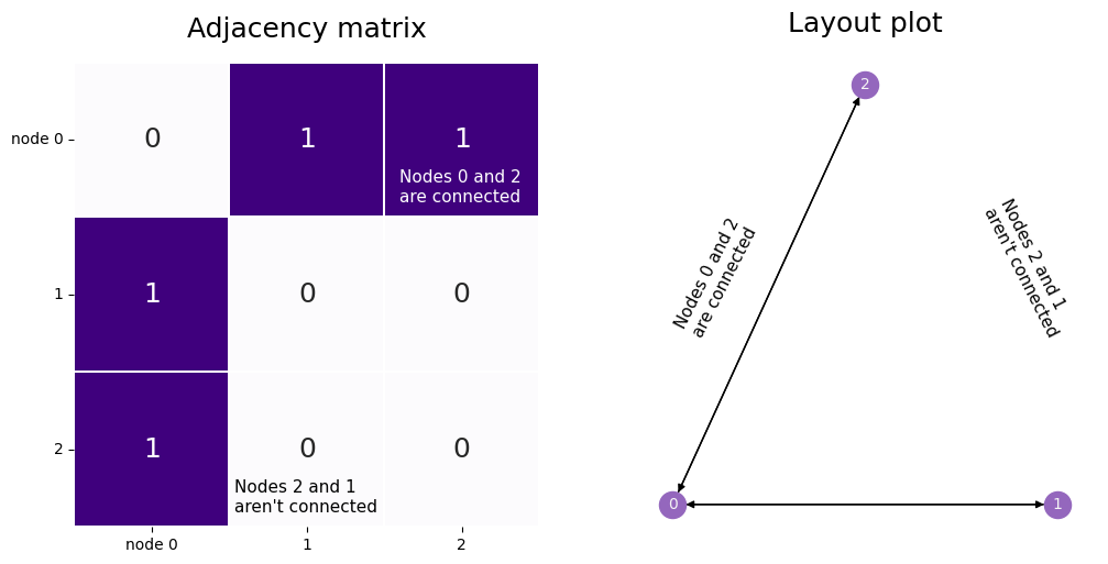
Our network has three nodes, labeled \(1\), \(2\), and \(3\). Each of these three nodes is either connected or not connected to each of the two other nodes. We’ll make a square matrix \(A\), with 3 rows and 3 columns, so that each node has its own row and column associated to it.

So, let’s fill out the matrix. We start with the first row, which corresponds to the first node, and move along the columns. If there is an edge between the first node and the node whose index matches the current column, put a 1 in the current location. If the two nodes aren’t connected, add a 0. When you’re done with the first row, move on to the second. Keep going until the whole matrix is filled with 0’s and 1’s.

The end result looks like the matrix below. Since the second and third nodes aren’t connected, there is a \(0\) in locations \(A_{2, 1}\) and \(A_{1, 2}\). There are also zeroes along the diagonals, since nodes don’t have edges with themselves.

from graphbook_code import heatmap
import matplotlib.pyplot as plt
import seaborn as sns

fig, axs = plt.subplots(1, 2, figsize=(12,6))
ax1 = heatmap(A, annot=True, linewidths=.1, cbar=False, ax=axs[0], title="Adjacency matrix", 
               xticklabels=True, yticklabels=True);
ax1.tick_params(axis='y', labelrotation=360)

# ticks
yticks = ax1.get_yticklabels()
yticks[0].set_text('node 0')
ax1.set_yticklabels(yticks)

xticks = ax1.get_xticklabels()
xticks[0].set_text('node 0')
ax1.set_xticklabels(xticks)

ax1.annotate("Nodes 0 and 2 \nare connected", (2.1, 0.9), color='white', fontsize=11)
ax1.annotate("Nodes 2 and 1 \naren't connected", (1.03, 2.9), color='black', fontsize=11)

ax2 = nx.draw_networkx(G, with_labels=True, node_color="tab:purple", pos=pos,
                font_size=10, font_color="whitesmoke", arrows=True, edge_color="black",
                width=1, ax=axs[1])

ax2 = plt.gca()
ax2.text(0, 0.2, s="Nodes 0 and 2 \nare connected", color='black', fontsize=11, rotation=63)
ax2.text(.8, .2, s="Nodes 2 and 1 \naren't connected", color='black', fontsize=11, rotation=-63)
ax2.set_title("Layout plot", fontsize=18)
sns.despine(ax=ax2, left=True, bottom=True)

Although the adjacency matrix is straightforward and easy to understand, it isn’t the only way to represent networks.

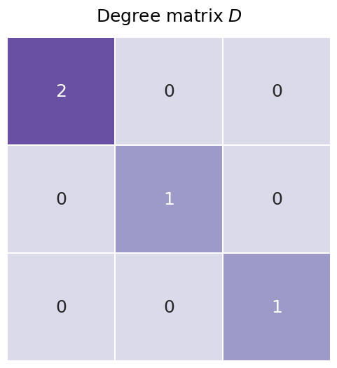
3.1.2. The Degree Matrix

The degree matrix isn’t a full representation of our network, because you wouldn’t be able to reconstruct an entire network from a degree matrix. However, it’s fairly straightforward and it pops up relatively often as a step in creating other matrices, so the degree matrix is useful to mention. It’s just a diagonal matrix with the values along the diagonal corresponding to the number of each edges each node has, also known as the degree of each node. You’ll learn more about the degree matrix in the next section Section 3.2.

You can see the degree matrix for our network below. The diagonal element corresponding to node zero has the value of two, since it has two edges; the rest of the nodes have a value of one, since they each are only connected to the first node.

# Build the degree matrix D
degrees = np.count_nonzero(A, axis=0)
D = np.diag(degrees)

fig, ax = plt.subplots(figsize=(6,6))

D_ax = heatmap(D, annot=True, linewidths=.1, cbar=False, title="Degree matrix $D$", 
               ax=ax);

3.1.3. The Laplacian Matrix

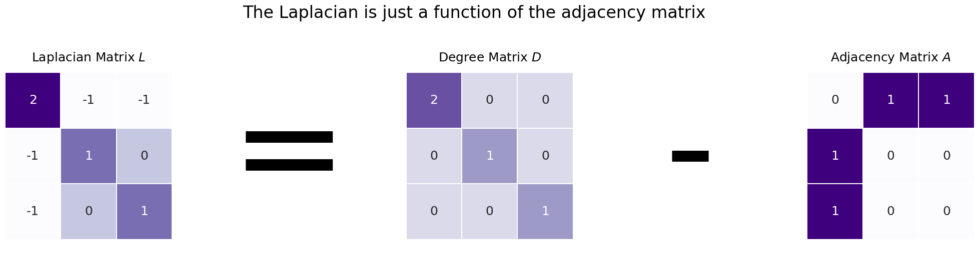
The standard, cookie-cutter Laplacian Matrix \(L\) [2] is just the adjacency matrix \(A\) subtracted from the the degree matrix \(D\):

\(L = D - A\)

Since the only nonzero values of the degree matrix is along its diagonals, and because the diagonals of an adjacency matrix never contain zeroes if its network doesn’t have nodes connected to themselves, the diagonals of the Laplacian are just the degree of each node. The values on the non-diagonals work similarly to the adjacency matrix: they contain a \(-1\) if there is an edge between the two nodes, and a \(0\) if there is no edge.

The figure below shows you what the Laplacian looks like. Since each node has exactly two edges, the degree matrix is just a diagonal matrix of all twos. The Laplacian looks like the degree matrix, but with -1’s in all the locations where an edge exists between nodes \(i\) and \(j\).

L = D - A

from graphbook_code import heatmap
import seaborn as sns
from matplotlib.colors import Normalize
from graphbook_code import GraphColormap
import matplotlib.cm as cm
import matplotlib.pyplot as plt

fig, axs = plt.subplots(1, 5, figsize=(25, 5))

# First axis (Laplacian)
L_ax = heatmap(L, ax=axs[0], cbar=False, title="Laplacian Matrix $L$", annot=True, 
        linewidths=.1)

# Second axis (-)
axs[1].text(x=.5, y=.5, s="=", fontsize=200, 
            va='center', ha='center')
axs[1].get_xaxis().set_visible(False)
axs[1].get_yaxis().set_visible(False)
sns.despine(ax=axs[1], left=True, bottom=True)

# Third axis (Degree matrix)

heatmap(D, ax=axs[2], cbar=False, title="Degree Matrix $D$", annot=True, 
        linewidths=.1)

# Third axis (=)
axs[3].text(x=.5, y=.5, s="-", fontsize=200,
            va='center', ha='center')
axs[3].get_xaxis().set_visible(False)
axs[3].get_yaxis().set_visible(False)
sns.despine(ax=axs[3], left=True, bottom=True)

# Fourth axis (Laplacian)
heatmap(A, ax=axs[4], cbar=False, title="Adjacency Matrix $A$", annot=True, 
        linewidths=.1)

fig.suptitle("The Laplacian is just a function of the adjacency matrix", fontsize=24, y=1.1);

We use the Laplacian in practice because it has a number of interesting mathematical properties, which tend to be useful for analysis. For instance, the magnitude of its second-smallest eigenvalue, called the Fiedler eigenvalue, tells you how well-connected your network is – and the number of eigenvalues equal to zero is the number of connected components your network has (a connected component is a group of nodes in a network which all have a path to get to each other – think of it as an island of nodes and edges). Incidentally, this means that the smallest eigenvalue of the Laplacian will always be 0, since any simple network always has at least one “island”.

Another interesting property of the Laplacian is that the sum of its diagonals is twice the number of edges in the network. Because the sum of the diagonal matrix is the trace, and the trace is also equal to the sum of the eigenvalues, this means that the sum of the eigenvalues of the Laplacian is equal to twice the number of edges in the network.

Laplacians and adjacency matrices will be used throughout this book, and details about when and where one or the other will be used are in the spectral embedding chapter.

3.1.3.1. The Normalized Laplacian

There are a few variations on the standard \(D-A\) version of the Laplacian which are widely used in practice, and which (confusingly) are often also called the Laplacian. They tend to have similar properties. The Normalized Laplacian, \(L^{normalized}\) is one such variation. The Normalized Laplacian [2] is defined as:

\(L^{normalized} = D^{-1/2} L D^{-1/2} = I - D^{-1/2} A D^{-1/2}\)

Where \(I\) is the identity matrix (the square matrix with all zeroes except for ones along the diagonal). You can work through the algebra yourself if you’d like to verify that the second expression is the same as the third.

Below you can see the normalized Laplacian in code. We use graspologic’s to_laplacian function, with the form set to I - DAD, which computes \(L^{normalized}\) above.

from graspologic.utils import to_laplacian
L_sym = to_laplacian(A, form="I-DAD")

fig, axs = plt.subplots(1, 2, figsize=(12,6))

L_sym_ax = heatmap(L_sym, annot=True, linewidths=.1, cbar=False, title="Normalized Laplacian $L^{normalized}$", 
               xticklabels=True, yticklabels=True, ax=axs[0]);

L_sym_ax.tick_params(axis='y', labelrotation=360)


ax2 = nx.draw_networkx(G, with_labels=True, node_color="tab:purple", pos=pos,
                font_size=10, font_color="whitesmoke", arrows=True, edge_color="black",
                width=1, ax=axs[1])

ax2 = plt.gca()
ax2.text(.24, 0.2, s="Edge 1", color='black', fontsize=11, rotation=65)
ax2.text(.45, 0.01, s="Edge 0", color='black', fontsize=11)
ax2.set_title("Layout plot", fontsize=18)
sns.despine(ax=ax2, left=True, bottom=True)

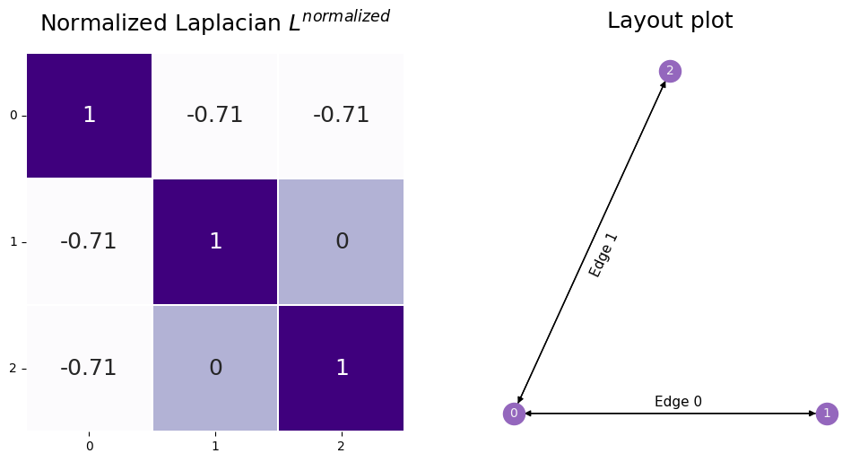
You can understand the normalized Laplacian from the name: you can think of it as the Laplacian normalized by the degrees of the nodes associated with a given entry.

You can see this by looking at what the operation is doing:

\[\begin{align*} L^{normalized} &= D^{-\frac{1}{2}}L D^{-\frac{1}{2}} \\ &= \begin{bmatrix} d_{1} & & \\ & \ddots & \\ & & d_n \end{bmatrix}^{-\frac{1}{2}}\begin{bmatrix} l_{11} & ... & l_{1n} \\ \vdots & \ddots & \vdots \\ l_{n1} & ... & l_{nn} \end{bmatrix} \begin{bmatrix} d_{1} & & \\ & \ddots & \\ & & d_n \end{bmatrix}^{-\frac{1}{2}} \\ &= \begin{bmatrix} \frac{1}{\sqrt{d_1}} & & \\ & \ddots & \\ & & \frac{1}{\sqrt{d_n}} \end{bmatrix}\begin{bmatrix} l_{11} & ... & l_{1n} \\ \vdots & \ddots & \vdots \\ l_{n1} & ... & l_{nn} \end{bmatrix} \begin{bmatrix} \frac{1}{\sqrt{d_1}} & & \\ & \ddots & \\ & & \frac{1}{\sqrt{d_n}} \end{bmatrix} \\ &= \begin{bmatrix} \frac{l_{11}}{d_1} & ... & \frac{l_{1n}}{\sqrt{d_1}\sqrt{d_n}} \\ \vdots & \ddots & \vdots \\ \frac{l_{n1}}{\sqrt{d_n}\sqrt{d_1}} & ... & \frac{l_{nn}}{d_n} \end{bmatrix} \end{align*}\]

So the normalized laplacian has entries \(l^{normalized}_{ij} = \frac{l_{ij}}{\sqrt{d_i}\sqrt{d_j}}\).

We can plug in the value of \(L\) to obtain a similar relationship with the adjacency matrix \(A\). Notice that:

\[\begin{align*} L^{normalized} &= D^{-\frac{1}{2}}L D^{-\frac{1}{2}} \\ &= D^{-\frac{1}{2}}(D - A) D^{-\frac{1}{2}} \\ &= D^{-\frac{1}{2}}DD^{-\frac{1}{2}} - D^{-\frac{1}{2}}A D^{-\frac{1}{2}} \\ &= D^{\frac{1}{2}}D^{-\frac{1}{2}} - D^{-\frac{1}{2}}A D^{-\frac{1}{2}} \\ &= I_{n \times n} - D^{-\frac{1}{2}}A D^{-\frac{1}{2}} \end{align*}\]

The \(D^{-1/2} D D^{-1/2}\) term is spiritually the same as what you’d think of \(\frac{D}{D}\) (if that was defined!), since it just works out to be the identity matrix. The \(D^{-1/2} A D^{-1/2}\) is just doing the same thing to \(A\) that you did to \(L\). So you’re normalizing the entries of the adjacency matrix by the degrees of the nodes a given entry is concerned with; that is, \(\frac{a_{ij}}{\sqrt{d_i}\sqrt{d_j}}\).

One useful property of the normalized Laplacian is that its eigenvalues are bounded between 0 and 2. This normalization tends to be useful, because the Laplacian is a thing called a positive semi-definite matrix. This means that a suite of linear algebra techniques, which may not run successfully on the adjacency matrix (which is not positive semi-definite in its most raw form for simple networks, which you will learn about in the next chapter), can be executed on the network Laplacian. For more details about the properties of the Laplacian, check out [3].

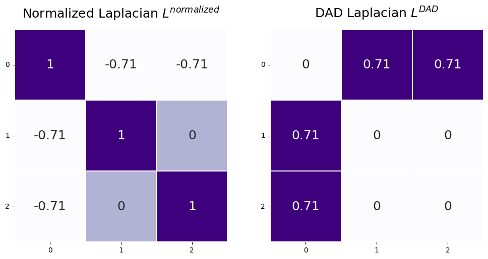
3.1.3.2. The DAD Laplacian

In this book, a lot of what we will cover will be something called a spectral embedding of the Laplacian. While you will learn all about this in Section 5.3, there are some fine points we want to cover here. As it turns out, there is another, related, definition of a Laplacian, which we call the DAD Laplacian:

\[\begin{align*} L^{DAD} &= D^{-\frac{1}{2}}A D^{-\frac{1}{2}} \end{align*}\]

\(L^{DAD}\) and \(L^{normalized}\) share some major similarities which are important to note here. Later in the book in Section 5.3, you will learn about the importance of the singular value decomposition for spectral embedding of Laplacians. Basically, what the singular value decomposition will allow you to do is look at the laplacian as a sum of much simpler matrices. By “simple”, what we mean here is that they can be represented as the product of two vectors, which the Laplacian, in general, cannot. By looking only at the first few of these “simple” matrices, you can learn about the Laplacian and reduce a lot of the noise in the Laplacian itself. The properties of looking at the DAD Laplacian are discussed at length in [4] and [5].

The most important connection is that these “simple” matrices will be identical for \(L^{normalized}\) and \(L^{DAD}\), except for one important fact: they will be in reverse order from one another. In \(L^{normalized}\), the matrices you will want to use will be the last few, and in \(L^{DAD}\), the matrices you will want to use will be the first few. When you compute the singular value decomposition, there are ways to only compute the first few matrices without having to go through the trouble of computing all of them, whereas the reverse is not true! To get the last few simple matrices, you would have to compute all of the preceding ones first. This means that to get the simple matrices you want, you can get much better computational performance using \(L^{DAD}\) instead of \(L^{normalized}\).

You can compute the \(L^{DAD}\) in graspologic similarly to above, but with form="DAD":

L_dad = to_laplacian(A, form="DAD")

fig, axs = plt.subplots(1, 2, figsize=(12,6))

L_sym_ax = heatmap(L_sym, annot=True, linewidths=.1, cbar=False, title="Normalized Laplacian $L^{normalized}$", 
               xticklabels=True, yticklabels=True, ax=axs[0]);

L_sym_ax.tick_params(axis='y', labelrotation=360)


L_dad_ax = heatmap(L_dad, annot=True, linewidths=.1, cbar=False, title="DAD Laplacian $L^{DAD}$", 
               xticklabels=True, yticklabels=True, ax=axs[1]);

L_dad_ax.tick_params(axis='y', labelrotation=360)

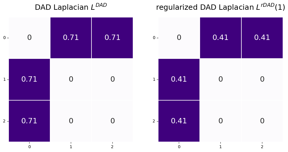
3.1.3.3. The regularized Laplacian

The regularized Laplacian is an adaptation of the DAD Laplacian you learned about in the previous section. As it turns out, when networks have degree matrices where some of the degrees are really, really small, the spectral clustering approach you will learn about in Section 5.3 is simply not going to perform very well. When we say it is not going to perform very well, what we mean is that the spectral clusterings are going to be extremely influenced by these nodes with really small node degrees. To overcome this hurdle, instead of using the DAD Laplacian, you can use the regularized Laplacian, defined extremely similarly to the DAD Laplacian, as:

\[\begin{align*} L^{rDAD}(\tau) &= D_\tau^{-\frac{1}{2}}A D_\tau^{-\frac{1}{2}} \end{align*}\]

Where \(\tau\) is a regularization constant which is greater than or equal to zero, and \(D_\tau = D + \tau I\). When we put \(\tau\) in parentheses here (that is, \((\tau)\)), all that we mean is that \(L^{rDAD}\) is a function of the particular regularization constant that you choose. Basically, what this is going to do is just “inflate” the diagonal elements of the degree matrix. So, if the degree for some of the nodes is extremely small, when we add a constant \(\tau\) to them, we can increase the degrees by \(\tau\). In effect, what this will do is make the nodes with really small degrees (which, like we said, might cause issues in the spectral clustering) a lot less impactful on the results that you obtain. Also, as you can see, if \(\tau = 0\), then \(L^{rDAD}(\tau) = L^{DAD}\). The regularized Laplacian is discussed at length in [6].

Let’s take a look at what \(L^{rDAD}(\tau)\) and \(L^{DAD}\) look like when we pick \(\tau\) to be \(1\). You can do this in graspologic using form="R-DAD", and then setting regularizer appropriately:

tau = 1
L_rdad = to_laplacian(A, form="R-DAD", regularizer=tau)

fig, axs = plt.subplots(1, 2, figsize=(12,6))


L_dad_ax = heatmap(L_dad, annot=True, linewidths=.1, cbar=False, title="DAD Laplacian $L^{DAD}$", 
               xticklabels=True, yticklabels=True, ax=axs[0]);

L_dad_ax.tick_params(axis='y', labelrotation=360)


L_dad_ax = heatmap(L_rdad, annot=True, linewidths=.1, cbar=False, title="regularized DAD Laplacian $L^{rDAD}(1)$", 
               xticklabels=True, yticklabels=True, ax=axs[1]);

L_dad_ax.tick_params(axis='y', labelrotation=360)

3.1.4. References

1

Chris Godsil and Gordon Royle. Algebraic Graph Theory. Springer, New York, NY, USA, 2001. ISBN 978-1-4613-0163-9. URL: https://link.springer.com/book/10.1007/978-1-4613-0163-9.

2(1,2)

Fan Chung. Spectral Graph Theory. Volume 92. American Mathematical Society, December 1996. ISBN 978-0-8218-0315-8. doi:10.1090/cbms/092.

3

Jianxi Li, Ji-Ming Guo, and Wai Chee Shiu. Bounds on normalized Laplacian eigenvalues of graphs. J. Inequal. Appl., 2014(1):1–8, December 2014. doi:10.1186/1029-242X-2014-316.

4

Kamalika Chaudhuri, Fan Chung, and Alexander Tsiatas. Spectral Clustering of Graphs with General Degrees in the Extended Planted Partition Model. In Conference on Learning Theory, pages 35.1–35.23. JMLR Workshop and Conference Proceedings, June 2012. URL: https://proceedings.mlr.press/v23/chaudhuri12.html.

5

Arash A. Amini, Aiyou Chen, Peter J. Bickel, and Elizaveta Levina. Pseudo-likelihood methods for community detection in large sparse networks. arXiv, July 2012. arXiv:1207.2340, doi:10.1214/13-AOS1138.

6

Tai Qin and Karl Rohe. Regularized Spectral Clustering under the Degree-Corrected Stochastic Blockmodel. arXiv, September 2013. arXiv:1309.4111, doi:10.48550/arXiv.1309.4111.