RDPGs and more general network models
Contents
11.6. RDPGs and more general network models#
11.6.1. Random Dot Product Graph (RDPG)#
11.6.1.1. A Priori RDPG#
The a priori Random Dot Product Graph is an RDPG in which we know a priori the latent position matrix \(X\). The a priori RDPG has the following parameter:
Parameter |
Space |
Description |
|---|---|---|
\(X\) |
\( \mathbb R^{n \times d}\) |
The matrix of latent positions for each node \(n\). |
\(X\) is called the latent position matrix of the RDPG. We write that \(X \in \mathbb R^{n \times d}\), which means that it is a matrix with real values, \(n\) rows, and \(d\) columns. We will use the notation \(\vec x_i\) to refer to the \(i^{th}\) row of \(X\). \(\vec x_i\) is referred to as the latent position of a node \(i\). This looks something like this:
Noting that \(X\) has \(d\) columns, this implies that \(\vec x_i \in \mathbb R^d\), or that each node’s latent position is a real-valued \(d\)-dimensional vector.
What is the generative model for the a priori RDPG? As we discussed above, given \(X\), for all \(j > i\), \(\mathbf a_{ij} \sim Bern(\vec x_i^\top \vec x_j)\) independently. If \(i < j\), \(\mathbf a_{ji} = \mathbf a_{ij}\) (the network is undirected), and \(\mathbf a_{ii} = 0\) (the network is loopless). If \(\mathbf A\) is an a priori RDPG with parameter \(X\), we write that \(\mathbf A \sim RDPG_n(X)\).
11.6.1.1.1. Probability#
Given \(X\), the probability for an RDPG is relatively straightforward, as an RDPG is another Independent-Edge Random Graph. The independence assumption vastly simplifies our resulting expression. We will also use many of the results we’ve identified above, such as the p.m.f. of a Bernoulli random variable. Finally, we’ll note that the probability matrix \(P = (\vec x_i^\top \vec x_j)\), so \(p_{ij} = \vec x_i^\top \vec x_j\):
Unfortunately, the probability equivalence classes are a bit harder to understand intuitionally here compared to the ER and SBM examples so we won’t write them down here, but they still exist!
11.6.1.2. A Posteriori RDPG#
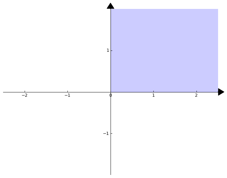
Like for the a posteriori SBM, the a posteriori RDPG introduces another strange set: the intersection of the unit ball and the non-negative orthant. Huh? This sounds like a real mouthful, but it turns out to be rather straightforward. You are probably already very familiar with a particular orthant: in two-dimensions, an orthant is called a quadrant. Basically, an orthant just extends the concept of a quadrant to spaces which might have more than \(2\) dimensions. The non-negative orthant happens to be the orthant where all of the entries are non-negative. We call the \(K\)-dimensional non-negative orthant the set of points in \(K\)-dimensional real space, where:
In two dimensions, this is the traditional upper-right portion of the standard coordinate axis. To give you a picture, the \(2\)-dimensional non-negative orthant is the blue region of the following figure:
import numpy as np
import matplotlib.pyplot as plt
from mpl_toolkits.axisartist import SubplotZero
import matplotlib.patches as patch

class myAxes():

    def __init__(self, xlim=(-5,5), ylim=(-5,5), figsize=(6,6)):
        self.xlim = xlim
        self.ylim = ylim
        self.figsize  = figsize
        self.__scale_arrows()
    def __drawArrow(self, x, y, dx, dy, width, length):
        plt.arrow(
            x, y, dx, dy,
            color       = 'k',
            clip_on     = False,
            head_width  = self.head_width,
            head_length = self.head_length
        )

    def __scale_arrows(self):
        """ Make the arrows look good regardless of the axis limits """
        xrange = self.xlim[1] - self.xlim[0]
        yrange = self.ylim[1] - self.ylim[0]

        self.head_width  = min(xrange/30, 0.25)
        self.head_length = min(yrange/30, 0.3)

    def __drawAxis(self):
        """
        Draws the 2D cartesian axis
        """
        # A subplot with two additional axis, "xzero" and "yzero"
        # corresponding to the cartesian axis
        ax = SubplotZero(self.fig, 1, 1, 1)
        self.fig.add_subplot(ax)

        # make xzero axis (horizontal axis line through y=0) visible.
        for axis in ["xzero","yzero"]:
            ax.axis[axis].set_visible(True)
        # make the other axis (left, bottom, top, right) invisible
        for n in ["left", "right", "bottom", "top"]:
            ax.axis[n].set_visible(False)

        # Plot limits
        plt.xlim(self.xlim)
        plt.ylim(self.ylim)
        ax.set_yticks([-1, 1, ])
        ax.set_xticks([-2, -1, 0, 1, 2])
        # Draw the arrows
        self.__drawArrow(self.xlim[1], 0, 0.01, 0, 0.3, 0.2) # x-axis arrow
        self.__drawArrow(0, self.ylim[1], 0, 0.01, 0.2, 0.3) # y-axis arrow
        self.ax=ax

    def draw(self):
        # First draw the axis
        self.fig = plt.figure(figsize=self.figsize)
        self.__drawAxis()

axes = myAxes(xlim=(-2.5,2.5), ylim=(-2,2), figsize=(9,7))
axes.draw()

rectangle =patch.Rectangle((0,0), 3, 3, fc='blue',ec="blue", alpha=.2)
axes.ax.add_patch(rectangle)
plt.show()
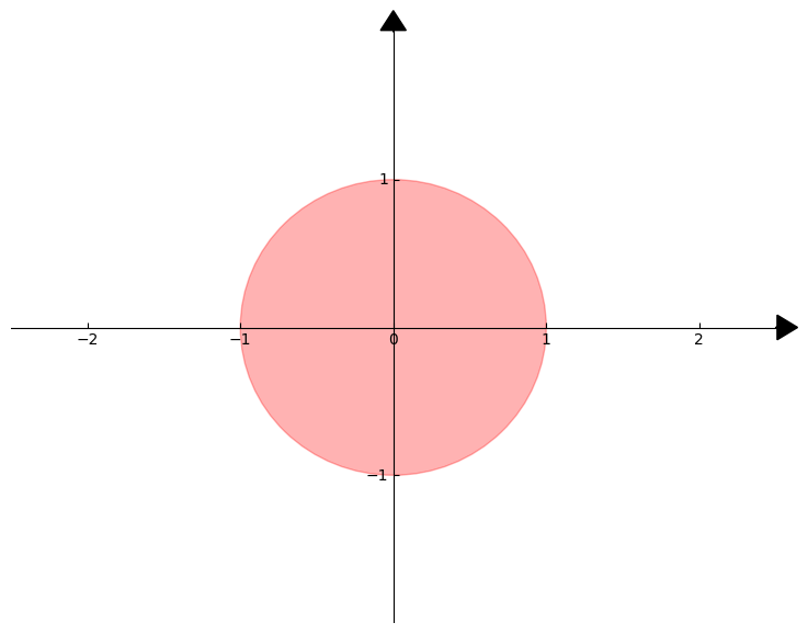
Now, what is the unit ball? You are probably familiar with the idea of the unit ball, even if you haven’t heard it called that specifically. Remember that the Euclidean norm for a point \(\vec x\) which has coordinates \(x_i\) for \(i=1,...,K\) is given by the expression:
The Euclidean unit ball is just the set of points whose Euclidean norm is at most \(1\). To be more specific, the closed unit ball with the Euclidean norm is the set of points:
We draw the \(2\)-dimensional unit ball with the Euclidean norm below, where the points that make up the unit ball are shown in red:
axes = myAxes(xlim=(-2.5,2.5), ylim=(-2,2), figsize=(9,7))
axes.draw()

circle =patch.Circle((0,0), 1, fc='red',ec="red", alpha=.3)
axes.ax.add_patch(circle)
plt.show()
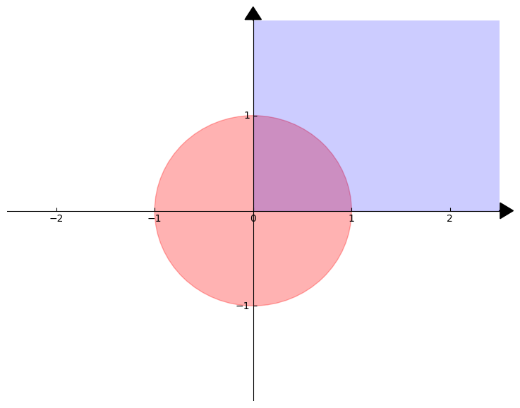
Now what is their intersection? Remember that the intersection of two sets \(A\) and \(B\) is the set:
That is, each element must be in both sets to be in the intersection. The interesction of the unit ball and the non-negative orthant will be the set:
visually, this will be the set of points in the overlap of the unit ball and the non-negative orthant, which we show below in purple:
axes = myAxes(xlim=(-2.5,2.5), ylim=(-2,2), figsize=(9,7))
axes.draw()

circle =patch.Circle((0,0), 1, fc='red',ec="red", alpha=.3)
axes.ax.add_patch(circle)
rectangle =patch.Rectangle((0,0), 3, 3, fc='blue',ec="blue", alpha=.2)
axes.ax.add_patch(rectangle)
plt.show()
This space has an incredibly important corollary. It turns out that if \(\vec x\) and \(\vec y\) are both elements of \(\mathcal X_K\), that \(\left\langle \vec x, \vec y \right \rangle = \vec x^\top \vec y\), the inner product, is at most \(1\), and at least \(0\). Without getting too technical, this is because of something called the Cauchy-Schwartz inequality and the properties of \(\mathcal X_K\). If you remember from linear algebra, the Cauchy-Schwartz inequality states that \(\left\langle \vec x, \vec y \right \rangle\) can be at most the product of \(\left|\left|\vec x\right|\right|_2\) and \(\left|\left|\vec y\right|\right|_2\). Since \(\vec x\) and \(\vec y\) have norms both less than or equal to \(1\) (since they are on the unit ball), their inner-product is at most \(1\). Further, since \(\vec x\) and \(\vec y\) are in the non-negative orthant, their inner product can never be negative. This is because both \(\vec x\) and \(\vec y\) have entries which are not negative, and therefore their element-wise products can never be negative.
The a posteriori RDPG is to the a priori RDPG what the a posteriori SBM was to the a priori SBM. We instead suppose that we do not know the latent position matrix \(X\), but instead know how we can characterize the individual latent positions. We have the following parameter:
Parameter |
Space |
Description |
|---|---|---|
F |
inner-product distributions |
A distribution which governs each latent position. |
The parameter \(F\) is what is known as an inner-product distribution. In the simplest case, we will assume that \(F\) is a distribution on a subset of the possible real vectors that have \(d\)-dimensions with an important caveat: for any two vectors within this subset, their inner product must be a probability. We will refer to the subset of the possible real vectors as \(\mathcal X_K\), which we learned about above. This means that for any \(\vec x_i, \vec x_j\) that are in \(\mathcal X_K\), it is always the case that \(\vec x_i^\top \vec x_j\) is between \(0\) and \(1\). This is essential because like previously, we will describe the distribution of each edge in the adjacency matrix using \(\vec x_i^\top \vec x_j\) to represent a probability. Next, we will treat the latent position matrix as a matrix-valued random variable which is latent (remember, latent means that we don’t get to see it in our real data). Like before, we will call \(\vec{\mathbf x}_i\) the random latent positions for the nodes of our network. In this case, each \(\vec {\mathbf x}_i\) is sampled independently and identically from the inner-product distribution \(F\) described above. The latent-position matrix is the matrix-valued random variable \(\mathbf X\) whose entries are the latent vectors \(\vec {\mathbf x}_i\), for each of the \(n\) nodes.
The model for edges of the a posteriori RDPG can be described by conditioning on this unobserved latent-position matrix. We write down that, conditioned on \(\vec {\mathbf x}_i = \vec x\) and \(\vec {\mathbf x}_j = \vec y\), that if \(j > i\), then \(\mathbf a_{ij}\) is sampled independently from a \(Bern(\vec x^\top \vec y)\) distribution. As before, if \(i < j\), \(\mathbf a_{ji} = \mathbf a_{ij}\) (the network is undirected), and \(\mathbf a_{ii} = 0\) (the network is loopless). If \(\mathbf A\) is the adjacency matrix for an a posteriori RDPG with parameter \(F\), we write that \(\mathbf A \sim RDPG_n(F)\).
11.6.1.2.1. Probability#
The probability for the a posteriori RDPG is fairly complicated. This is because, like the a posteriori SBM, we do not actually get to see the latent position matrix \(\mathbf X\), so we need to use integration to obtain an expression for the probability. Here, we are concerned with realizations of \(\mathbf X\). Remember that \(\mathbf X\) is just a matrix whose rows are \(\vec {\mathbf x}_i\), each of which individually have have the distribution \(F\); e.g., \(\vec{\mathbf x}_i \sim F\) independently. For simplicity, we will assume that \(F\) is a disrete distribution on \(\mathcal X_K\). This makes the logic of what is going on below much simpler since the notation gets less complicated, but does not detract from the generalizability of the result (the only difference is that sums would be replaced by multivariate integrals, and probability mass functions replaced by probability density functions).
We will let \(p\) denote the probability mass function (p.m.f.) of this discrete distribution function \(F\). The strategy will be to use the independence assumption, followed by integration over the relevant rows of \(\mathbf X\):
Next, we will simplify this expression a little bit more, using the definition of a conditional probability like we did before for the SBM:
Further, remember that if \(\mathbf a\) and \(\mathbf b\) are independent, then \(Pr(\mathbf a = a, \mathbf b = b) = Pr(\mathbf a = a)Pr(\mathbf b = b)\). Using that \(\vec x_i\) and \(\vec x_j\) are independent, by definition:
Which means that:
Finally, we that conditional on \(\vec{\mathbf x}_i = \vec x_i\) and \(\vec{\mathbf x}_j = \vec x_j\), \(\mathbf a_{ij}\) is \(Bern(\vec x_i^\top \vec x_j)\). This means that in terms of our probability matrix, each entry \(p_{ij} = \vec x_i^\top \vec x_j\). Therefore:
This implies that:
So our complete expression for the probability is:
11.6.2. Generalized Random Dot Product Graph (GRDPG)#
The Generalized Random Dot Product Graph, or GRDPG, is the most general random network model we will consider in this book. Note that for the RDPG, the probability matrix \(P\) had entries \(p_{ij} = \vec x_i^\top \vec x_j\). What about \(p_{ji}\)? Well, \(p_{ji} = \vec x_j^\top \vec x_i\), which is exactly the same as \(p_{ij}\)! This means that even if we were to consider a directed RDPG, the probabilities that can be captured are always going to be symmetric. The generalized random dot product graph, or GRDPG, relaxes this assumption. This is achieved by using two latent positin matrices, \(X\) and \(Y\), and letting \(P = X Y^\top\). Now, the entries \(p_{ij} = \vec x_i^\top \vec y_j\), but \(p_{ji} = \vec x_j^\top \vec y_i\), which might be different.
11.6.2.1. A Priori GRDPG#
The a priori GRDPG is a GRDPG in which we know a priori the latent position matrices \(X\) and \(Y\). The a priori GRDPG has the following parameters:
Parameter |
Space |
Description |
|---|---|---|
\(X\) |
\( \mathbb R^{n \times d}\) |
The matrix of left latent positions for each node \(n\). |
\(Y\) |
\( \mathbb R^{n \times d}\) |
The matrix of right latent positions for each node \(n\). |
\(X\) and \(Y\) behave nearly the same as the latent position matrix \(X\) for the a priori RDPG, with the exception that they will be called the left latent position matrix and the right latent position matrix respectively. Further, the vectors \(\vec x_i\) will be the left latent positions, and \(\vec y_i\) will be the right latent positions, for a given node \(i\), for each node \(i=1,...,n\).
What is the generative model for the a priori GRDPG? As we discussed above, given \(X\) and \(Y\), for all \(j \neq i\), \(\mathbf a_{ij} \sim Bern(\vec x_i^\top \vec y_j)\) independently. If we consider only loopless networks, \(\mathbf a_{ij} = 0\). If \(\mathbf A\) is an a priori GRDPG with left and right latent position matrices \(X\) and \(Y\), we write that \(\mathbf A \sim GRDPG_n(X, Y)\).
11.6.2.2. A Posteriori GRDPG#
The A Posteriori GRDPG is very similar to the a posteriori RDPG. We have two parameters:
Parameter |
Space |
Description |
|---|---|---|
F |
inner-product distributions |
A distribution which governs the left latent positions. |
G |
inner-product distributions |
A distribution which governs the right latent positions. |
Here, we treat the left and right latent position matrices as latent variable matrices, like we did for a posteriori RDPG. That is, the left latent positions are sampled independently and identically from \(F\), and the right latent positions \(\vec y_i\) are sampled independently and identically from \(G\).
The model for edges of the a posteriori RDPG can be described by conditioning on the unobserved left and right latent-position matrices. We write down that, conditioned on \(\vec {\mathbf x}_i = \vec x\) and \(\vec {\mathbf y}_j = \vec y\), that if \(j \neq i\), then \(\mathbf a_{ij}\) is sampled independently from a \(Bern(\vec x^\top \vec y)\) distribution. As before, assuming the network is loopless, \(\mathbf a_{ii} = 0\). If \(\mathbf A\) is the adjacency matrix for an a posteriori RDPG with parameter \(F\), we write that \(\mathbf A \sim GRDPG_n(F, G)\).
11.6.3. Inhomogeneous Erdös-Rényi (IER)#
In the preceding models, we typically made assumptions about how we could characterize the edge-existence probabilities using fewer than \(\binom n 2\) different probabilities (one for each edge). The reason for this is that in general, \(n\) is usually relatively large, so attempting to actually learn \(\binom n 2\) different probabilities is not, in general, going to be very feasible (it is never feasible when we have a single network, since a single network only one observation for each independent edge). Further, it is relatively difficult to ask questions for which assuming edges share nothing in common (even if they don’t share the same probabilities, there may be properties underlying the probabilities, such as the latent positions that we saw above with the RDPG, that we might still want to characterize) is actually favorable.
Nonetheless, the most general model for an independent-edge random network is known as the Inhomogeneous Erdös-Rényi (IER) Random Network. An IER Random Network is characterized by the following parameters:
Parameter |
Space |
Description |
|---|---|---|
\(P\) |
[0,1]\(^{n \times n}\) |
The edge probability matrix. |
The probability matrix \(P\) is an \(n \times n\) matrix, where each entry \(p_{ij}\) is a probability (a value between \(0\) and \(1\)). Further, if we restrict ourselves to the case of simple networks like we have done so far, \(P\) will also be symmetric (\(p_{ij} = p_{ji}\) for all \(i\) and \(j\)). The generative model is similar to the preceding models we have seen: given the \((i, j)\) entry of \(P\), denoted \(p_{ij}\), the edges \(\mathbf a_{ij}\) are independent \(Bern(p_{ij})\), for any \(j > i\). Further, \(\mathbf a_{ii} = 0\) for all \(i\) (the network is loopless), and \(\mathbf a_{ji} = \mathbf a_{ij}\) (the network is undirected). If \(\mathbf A\) is the adjacency maatrix for an IER network with probability matarix \(P\), we write that \(\mathbf A \sim IER_n(P)\).
It is worth noting that all of the preceding models we have discussed so far are special cases of the IER model. This means that, for instance, if we were to consider only the probability matrices where all of the entries are the same, we could represent the ER models. Similarly, if we were to only to consider the probability matrices \(P\) where \(P = XX^\top\), we could represent any RDPG.
The IER Random Network can be thought of as the limit of Stochastic Block Models, as the number of communities equals the number of nodes in the network. Stated another way, an SBM Random Network where each node is in its own community is equivalent to an IER Random Network. Under this formulation, note that the block matarix for such an SBM, \(B\), would have \(n \times n\) unique entries. Taking \(P\) to be this block matrix shows that the IER is a limiting case of SBMs.
11.6.3.1. Probability#
The probability for a network which is IER is very straightforward. We use the independence assumption, and the p.m.f. of a Bernoulli-distributed random-variable \(\mathbf a_{ij}\):