7.1. Latent Two-Sample Hypothesis Testing

We have learned a lot thus far about network statistics, and now we want to apply some of that knowledge to doing two-sample network testing. Imagine you are part of an alien race called the Moops. You live in harmony with another race, called the Moors, that look very similar to you, on the planet Zinthar. The evil overlord Zelu takes a random number of Moops and Moors and puts them on an island. You want to find your fellow Moops, but the Moops and Moors look very similar to each other. However, you guess that, perhaps, if you were able to look at a network representing the brain connections for a Moop and another network representing the brain connections for a Moor, you think that there might be a difference between the two. What do you do?

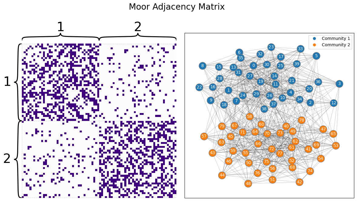
To make this a little bit more concrete, let’s develop our example. The Moops and Moors each have brains with $n=100$ brain areas. If two areas of the brain can communicate with one another (pass information back and forth), an edge exists; if they cannot communicate with one another, an edge does not exist. In this case, these networks will each be SBMs. The networks look like this:

from graspologic.simulations import sbm

ns = [40, 40]
BMoor = [[0.4, 0.1], [0.1, 0.4]]

AMoor = sbm(ns, BMoor, directed=False, loops=False)
zvec = ["1" for i in range(0, ns[0])] + ["2" for i in range(0, ns[1])]

Click to show

from graphbook_code import draw_multiplot

draw_multiplot(AMoor, labels=zvec, title="Moor Adjacency Matrix");

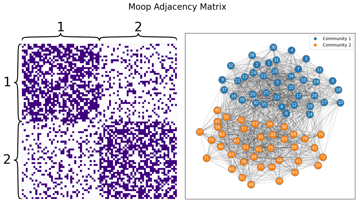
BMoop = [[0.6, 0.2], [0.2, 0.6]]

AMoop = sbm(ns, BMoop, directed=False, loops=False)

Click to show

draw_multiplot(AMoop, labels=zvec, title="Moop Adjacency Matrix");

7.1.1. Two-sample tests, a quick refresher

This problem is another iteration of a question you encountered in the last section when testing for differences between groups of edges from Section 6.2, called the two-sample test. You have two samples of data: a network from a Moop and a network from a Moor, and you want to characterize whether these two networks are different. For our purposes, you will call the Moop network $A^{(p)}$ and the Moor network $A^{(r)}$. As you by this time know, for each of these networks, there are underlying random networks, ${\mathbf{A}}^{(p)}$ and ${\mathbf{A}}^{(r)}$ of which the Moop and Moor networks you see, $A^{(p)}$ and $A^{(r)}$, are realizations of. The key issue is that you don’t actually get to see the underlying random networks: what you will need to do is characterize differences between ${\mathbf{A}}^{(p)}$ and ${\mathbf{A}}^{(r)}$ using only $A^{(p)}$ and $A^{(r)}$.

Since ${\mathbf{A}}^{(p)}$ and ${\mathbf{A}}^{(r)}$ are random, you can’t really study them directly. But what you can study, as it turns out, are the parameters that govern ${\mathbf{A}}^{(p)}$ and ${\mathbf{A}}^{(r)}$.

This is just like how, in our coin flip example you learned about previously, you don’t look for differences in the coins themselves, but rather, you look for differences in the probabilities that each coin lands on heads or tails. You construct hypotheses about the probabilities, not the coin. This is because the coins are the same (they both have a heads and tails side, all of the coin flips are performed without regard for the outcomes of other coin flips, so on and so forth), other than the fact that they land on heads and tails at different rates. This rate, the underlying probability, is therefore the element of the random coin that you want to hone in on to test whether they are different. Remember, you made a null hypothesis that there was no difference between the probabilities coins, $H_0:p_1=p_2$, and had an alternative hypothesis that there was a difference between the probabilities of the coins, $H_A:p_1\ne p_2$. Next, you produced estimates of the coin probabilities using the samples, ${\hat{p}}_1$ and ${\hat{p}}_2$, and then used the samples to deduce whether you have enough evidence from our sample to support whether $H_A$ was true, that $p_1\ne p_2$.

7.1.1.1. Two-sample tests and Random Networks

In this example, however, we’re going to go a slightly different direction. We’re going to describe ${\mathbf{A}}^{(p)}$ and ${\mathbf{A}}^{(r)}$ as Random Dot Product Graphs (RDPGs). What we’re going to say is that ${\mathbf{A}}^{(p)}$ is a random network where the probability an edge exists (or does not exist) is described by the probability matrix $P^{(p)}$, whose entries $p_{ij}^{(p)}$ are the probabilities that the edge ${\mathbf{a}}_{ij}^{(p)}$ between nodes $i$ and $j$ exist. You do the same thing for the Moor random network ${\mathbf{A}}^{(r)}$, with the probability matrix $P^{(r)}$.

In this case, you want to test whether $H_0:P^{(p)}=P^{(r)}$ against $H_A:P^{(p)}\ne P^{(r)}$. However, you have a slight problem: unlike the coin, you can’t really use your sample to describe $P^{(p)}$ and $P^{(r)}$ directly. Instead, you need to make assumptions about the random networks in order to learn things about them, which was why we introduced statistical models in Section 4. You first need to choose a statistical model to describe ${\mathbf{A}}^{(p)}$ and ${\mathbf{A}}^{(r)}$.

7.1.1.2. Assuming a statistical model

To test whether the probability matrices are different, we’re going to make the assumption that ${\mathbf{A}}^{(p)}$ and ${\mathbf{A}}^{(r)}$ are each Random Dot Product Graphs (RDPGs), with latent position matrices $X^{(p)}$ and $X^{(r)}$, respectively. Remember that for a RDPG with latent position matrix $X$, that the probability matrix $P=X{X}^{\mathrm{\top }}$. What this means is that if $P^{(p)}=X^{(p)}{X}^{(p)\mathrm{\top }}$ and $P^{(r)}=X^{(r)}{X}^{(r)\mathrm{\top }}$, then $P^{(p)}$ and $P^{(r)}$ are the same/different if $X^{(p)}$ and $X^{(r)}$ are same/different, right?

Unfortunately, this assumption is a close, but not quite correct. Remember back in Section 5 we introduced the idea of a rotation matrix in Section 5.3.6.1 with respect to the non-identifiability problem. As it turns out, for a rotation matrix $W$ which is $d\times d$, then $W{W}^{\mathrm{\top }}=I_{d\times d}$, the $d\times d$ identity matrix, which is the equivalent of multiplying by one for matrices. This means that any matrix times the identity matrix is just itself. So what if $X^{(p)}$ and $X^{(r)}$ are just rotations of each other? Stated another way, what if $X^{(p)}=X^{(r)}W$; that is, $X^{(p)}$ is just $X^{(r)}$, but rotated around?

Even if $X^{(r)}$ and $X^{(p)}$ are different, as long as they are just rotations of one another, then the probability matrices are identical. This is because, if we call $P^{(r)}=X^{(r)}{X}^{(r)\mathrm{\top }}$, then:

$$\begin{array}{rl}{P}^{(p)}& =X^{(p)}{X}^{(p)\mathrm{\top }},\\ & =X^{(r)}W{W}^{\mathrm{\top }}{X}^{(r)\mathrm{\top }},\text{we used that }{X}^{(r)}=X^{(p)}W\\ & =X^{(r)}{I}_{d\times d}{X}^{(r)\mathrm{\top }},\text{we used that }W\text{ is a rotation, so }W{W}^{\mathrm{\top }}=I_{d\times d}\\ & =X^{(r)}{X}^{(r)\mathrm{\top }}=P^{(r)}\end{array}$$

Which shows that the probability matrices would still actually be the same!

What this means for you is that you can’t just compare the latent position matrices, but rather, you have to compare the latent position matrices for any possible rotation matrix! Stated another way, we would say that $P^{(p)}$ and $P^{(r)}$ are equal if $X^{(r)}$ can be obtained by rotating $X^{(p)}$, and they are not equal if $X^{(r)}$ cannot be obtained by rotation $X^{(p)}$. We write this down as a hypothesis by saying that $H_0:X^{(p)}=X^{(r)}W$ for any rotation matrix $W$, against $H_A:X^{(p)}\ne X^{(r)}W$ for any rotation matrix $W$. With the assumption that ${\mathbf{A}}^{(p)}$ and ${\mathbf{A}}^{(r)}$ are RDPGs, this is exactly the same as saying that $H_0:P^{(p)}=P^{(r)}$, against $H_A:P^{(p)}\ne P^{(r)}$, which was our original statement we wanted to test.

7.1.2. Latent position test

So, now we are ready to get to implementing your idea. You have two random networks, ${\mathbf{A}}^{(p)}$ and ${\mathbf{A}}^{(r)}$, and you assume that they are both RDPGs with latent position matrices $X^{(p)}$ and $X^{(r)}$ respectively. You want to test whether the latent position matrices are the same up to a rotation, $H_0:X^{(p)}=X^{(r)}W$ for some rotation $W$, or they are different for any possible rotation $W$ $H_A:X^{(p)}\ne X^{(r)}W$.

To do this, the first step is to figure out whether $X^{(p)}$ and $X^{(r)}$ are rotations of one another. We do this by first trying to find the best possible rotation of $X^{(r)}$ to $X^{(p)}$. The problem can be written down as follows:

$$\begin{array}{r}\text{find }W\text{ where }||X^{(p)}-X^{(r)}W|{|}_F\text{ is minimized}\end{array}$$

The term $||A-B|{|}_F$ is the Frobenius distance, which you learned about in Definition 5.2 from Section 5.3.

Basically, the idea is that if $X^{(p)}$ and $X^{(r)}$ are rotations of one another (or close to it), then if you can find the right rotation $W$, then $X^{(p)}$ and $X^{(r)}W$ will be identical (and $||X^{(p)}-X^{(r)}W|{|}_F$ will be zero) or nearly identical (and $||X^{(p)}-X^{(r)}W|{|}_F$ will be small). If they are not rotations of one another, then this equation $||X^{(p)}-X^{(r)}W|{|}_F$ is going to have a comparatively high value, no matter what value of $W$ you could choose. This is called the orthogonal procrustes problem [1], and there are a variety of ways you can come up with a pretty good guess at what $W$ is, but we won’t need to go into details for our purposes.

Next, you need to figure out how to actually use this to implement a statitical test $H_0:X^{(p)}=X^{(r)}W$ against $H_A:X^{(p)}\ne X^{(r)}W$. You can estimate starting values for $X^{(p)}$ and $X^{(r)}$, by just using adjacency spectral embedding in Section 5.3. This gives you ${\hat{X}}^{(p)}$ and ${\hat{X}}^{(r)}$, respectively, which are your estimates of the latent position matrices.

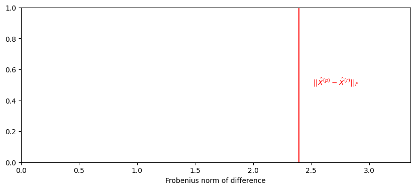
Next, you do your best to find a rotation of $X^{(r)}$ onto $X^{(p)}$ by solving the orthogonal procrustes problem, by plugging in your estimates ${\hat{X}}^{(p)}$ and ${\hat{X}}^{(r)}$ for $X^{(p)}$ and $X^{(r)}$. Unfortunately, you’re not going to find a matrix $W$ where $||{\hat{X}}^{(p)}-{\hat{X}}^{(r)}W|{|}_F=0$, even if $X^{(p)}$ and $X^{(r)}$ really are equal. This is because you are just using estimates of latent positions, so even if $X^{(p)}$ and $X^{(r)}$ are identical up to a rotation in reality, your estimates probably won’t be. This means that $||{\hat{X}}^{(p)}-{\hat{X}}^{(r)}W|{|}_F$ is, if ${\hat{X}}^{(p)}$ and ${\hat{X}}^{(r)}$ are close up to a rotation, going to take a relatively small value:

from scipy.linalg import orthogonal_procrustes
from graspologic.models import RDPGEstimator
import numpy as np

d = 2
# estimate latent positions for Moop and Moor networks
XMoop = RDPGEstimator(n_components=d).fit(AMoop).latent_
XMoor = RDPGEstimator(n_components=d).fit(AMoor).latent_
# estimate best possible rotation of XMoor to XMoop by 
# solving orthogonal procrustes problem
W = orthogonal_procrustes(XMoop, XMoor)[0]
observed_norm = np.linalg.norm(XMoop - XMoor @ W)

Click to show

from matplotlib import pyplot as plt
import seaborn as sns

fig, ax = plt.subplots(1, 1, figsize=(10, 4))
ax.set_title("")
ax.set_ylabel("")
ax.axvline(observed_norm, color="red")
ax.text(1.05*observed_norm , .5, "$||\\hat X^{(p)} - \\hat X^{(r)}||_F$", color="red");
ax.set_xlim([0, 1.4*observed_norm])
ax.set_xlabel("Frobenius norm of difference");

Relative what, exactly?

7.1.2.1. Generating a null distribution via parametric bootstrapping

In an ideal world, you would be able to characterize how far apart the estimates ${\hat{X}}^{(p)}$ and ${\hat{X}}^{(r)}$ would be if the quantities they were estimating, $X^{(p)}$ and $X^{(r)}$, were really identical up to a rotation. However, in reality, you don’t know $X^{(p)}$ nor $X^{(r)}$, so you can’t exactly say anything directly about how big $||{\hat{X}}^{(p)}-{\hat{X}}^{(r)}W|{|}_F$ should be if $X^{(p)}$ and $X^{(r)}$ are identical up to a rotation (and $H_0$ is true). If you did, you wouldn’t need to do any of this statistical testing in the first place!

So what you do is the next best thing. You instead use ${\hat{X}}^{(p)}$ as the parameter to generate two new networks, $A^{(1)}$ and $A^{(2)}$, where the latent positions really are identical (and equal to ${\hat{X}}^{(p)}$):

from graspologic.simulations import rdpg

def generate_synthetic_networks(X):
    """
    A function which generates two synthetic networks with
    same latent position matrix X.
    """
    A1 = rdpg(X, directed=False, loops=False)
    A2 = rdpg(X, directed=False, loops=False)
    return A1, A2

A1, A2 = generate_synthetic_networks(XMoop)

You then estimate the latent positions ${\hat{X}}^{(1)}$ and ${\hat{X}}^{(2)}$ using Adjacency Spectral Embedding again, and now you compute the value of $||{\hat{X}}^{(1)}-{\hat{X}}^{(2)}{W}_i|{|}_F$ for the best possible rotation $W_i$ of $X^{(2)}$ onto ${\hat{X}}^{(1)}$:

def compute_latent(A, d):
    """
    A function which returns the latent position estimate
    for an adjacency matrix A.
    """
    return RDPGEstimator(n_components=d).fit(A).latent_

X1 = compute_latent(A1, d)
X2 = compute_latent(A2, d)

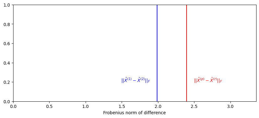
Finally, you compare $||{\hat{X}}^{(p)}-{\hat{X}}^{(r)}{W}_i|{|}_F$ to $||{\hat{X}}^{(1)}-{\hat{X}}^{(2)}W|{|}_F$. If $X^{(p)}$ and $X^{(r)}$ are identical up to a rotation, then you would expect that $||{\hat{X}}^{(p)}-{\hat{X}}^{(r)}W|{|}_F$ would be similar to $||{\hat{X}}^{(1)}-{\hat{X}}^{(2)}{W}_i|{|}_F$. If they are not, you would expect that $||{\hat{X}}^{(p)}-{\hat{X}}^{(r)}W|{|}_F$ would be much bigger than $||{\hat{X}}^{(1)}-{\hat{X}}^{(2)}{W}_i|{|}_F$:

def compute_norm_orth_proc(A, B):
    """
    A function which finds the best rotation of B onto A,
    and then computes and returns the norm.
    """
    R = orthogonal_procrustes(A, B)[0]
    return np.linalg.norm(A - B @ R)

norm_null = compute_norm_orth_proc(X1, X2)

Click to show

fig, ax = plt.subplots(1, 1, figsize=(10, 4))
ax.set_title("")
ax.set_ylabel("")
ax.axvline(observed_norm, color="red")
ax.text(observed_norm + .1, .2, "$||\\hat X^{(p)} - \\hat X^{(r)}||_F$", color="red")
ax.axvline(norm_null, color="blue")
ax.text(norm_null -.5, .2, "$||\\hat X^{(1)} - \\hat X^{(2)}||_F$", color="blue")
ax.set_xlim([0, 1.4*observed_norm])
ax.set_xlabel("Frobenius norm of difference");

You keep repeating this process again and again, and over time, you gradually get some idea of what $||{\hat{X}}^{(p)}-{\hat{X}}^{(r)}W|{|}_F$ would look like if the true latent position estimates were identical. This is called a parametric resampling. It is called a resampling because you are sampling what $||{\hat{X}}^{(1)}-{\hat{X}}^{(2)}{W}_i|{|}_F$ looks like if an assumption were true; namely, if the underlying latent position matrices were the same. It is called parametric because you are using properties of RDPGs to generate your estimates ${\hat{X}}^{(1)}$ and ${\hat{X}}^{(2)}$. When you do this dozens (or more) times, you start to notice a trend developing. We’ll plot what $||{\hat{X}}^{(1)}-{\hat{X}}^{(2)}{W}_i|{|}_F$ looks like when we repeat this process $100$ times using a histogram, which indicates the number of times the value of $||{\hat{X}}^{(1)}-{\hat{X}}^{(2)}{W}_i|{|}_F$ lands in a particular range of the $x$-axis:

def parametric_resample(A1, A2, d, nreps=100):
    """
    A function to generate samples of the null distribution under H0
    using parametric resampling.
    """
    null_norms = np.zeros(nreps)
    for i in range(0, nreps):
        A1, A2 = generate_synthetic_networks(XMoop)
        X1 = compute_latent(A1, d)
        X2 = compute_latent(A2, d)
        null_norms[i] = compute_norm_orth_proc(X1, X2)
    return null_norms

nreps = 100
null_norms = parametric_resample(AMoop, AMoor, 2, nreps=nreps)

Click to show

from pandas import DataFrame

samples = [{"Sample": i, "Norm": x} for i, x in enumerate(null_norms)]

null_df = DataFrame(samples)

fig, ax = plt.subplots(1, 1, figsize=(10, 4))
sns.histplot(null_df, x="Norm", stat="probability", ax=ax)
ax.axvline(observed_norm, color="red")
ax.set_xlim([0, 1.4*observed_norm])
ax.set_ylabel("Fraction of samples")
ax.text(np.median(null_norms) - .6, .2, "$||\\hat X^{(1)} - \\hat X^{(2)}||_F$", color="blue")
ax.text(observed_norm + .1, .2, "$||\\hat X^{(p)} - \\hat X^{(r)}||_F$", color="red");

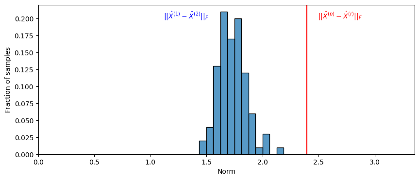
What you see is that $||{\hat{X}}^{(p)}-{\hat{X}}^{(r)}W|{|}_F$ is much larger than the almost all of the values of $||{\hat{X}}^{(1)}-{\hat{X}}^{(2)}{W}_i|{|}_F$ that you calculated. We will use this to estimate a $p$-value, and we will say that the $p$-value of $H_0$ against $H_A$ is the fraction of times that when the underlying latent positions were equal, the value of $||{\hat{X}}^{(1)}-{\hat{X}}^{(2)}{W}_i|{|}_F$ exceeded the value of $||{\hat{X}}^{(p)}-{\hat{X}}^{(r)}W|{|}_F$ which we estimated from our sample. We add one to the numerator and denominator, since we observed one instance of a value at least as big as that in the observed data: the observed data itself. This means our $p$-value is:

pval = ((null_norms >= observed_norm).sum() + 1)/(nreps + 1)
print("estimate of p-value: {:.3f}".format(pval))

estimate of p-value: 0.010

We then repeat this process, but we use $X^{(r)}$ instead as our reference point. The overall $p$-value is the maximum of the two $p$-values produced with this procedure.

This is called the latent position test, and it is implemented directly by graspologic. Note that the $p$-value that you obtain from this process might differ every time you run the test, since there is randomness in your generation process of the $A^{(1)}$s and the $A^{(2)}$s for every time you repeated your comparison. Making the number of repetitions larger by setting n_bootstraps to a higher value will tend to yield more stable $p$-value estimates for when we estimate $p$-values using resampling techniques:

from graspologic.inference import latent_position_test

nreps = 1000 # the number of times to repeat the process of estimating X1hat and X2hat
lpt_moop2moor = latent_position_test(AMoop, AMoor, n_bootstraps = nreps, n_components=d)
print("estimate of p-value: {:.5f}".format(lpt_moop2moor[1]))

estimate of p-value: 0.00100

The $p$-value is low, and below a typical decision threshold of $\alpha =0.05$. This means you have evidence to reject the null hypothesis in favor of the alternative hypothesis: the latent position matrix for a Moop brain network differs from the latent position matrix for a Moor brain network.

What if we had another network from a Moop, and we compared the network of our first Moop to our new Moop? We can generate a new comparison:

# generate a new Moor network with the same block matrix, and hence, 
# the same latent position matrix as AMoor
np.random.seed(1234)
AMoor2 = sbm(ns, BMoor)

lpt_moor2moor = latent_position_test(AMoor, AMoor2, n_bootstraps=nreps, n_components=d)
print("estimate of p-value: {:.5f}".format(lpt_moor2moor[1]))

estimate of p-value: 0.19580

The $p$-value is relatively large, so with $\alpha =0.05$, you fail to be able to reject the null hypothesis that the two Moops have the same latent position matrices. This process is described in [2].

7.1.3. Latent distribution test

To motivate a latent distribution test, we’re going to return to yet another coin example. Imagine that you and a friend do not each have a single coin like the examples that you have seen so far, but you each have a container of $300$ coins. Each of these $300$ coins can be identified as the coin ${\mathbf{x}}_i^{(y)}$ or ${\mathbf{x}}_i^{(f)}$, your $i^{th}$ coin or your friend’s $i^{th}$ coin. The outcomes ${\mathbf{x}}_i^{(y)}$ and ${\mathbf{x}}_i^{(f)}$ are random. These coins all have different probabilities of landing on heads, ${\mathbf{p}}_i^{(y)}$ and ${\mathbf{p}}_i^{(f)}$, again for your coin and your friend’s coin, respectively, and the probabilities that the coins land on heads is random too! Let’s say, for sake of example, that your coins have probabilities of landing on heads that tend to be right around $\frac{3}{8}$, but your friend’s coins have probabilities of landing on heads right around $\frac{5}{8}$:

ncoins = 300  # the number of coins in each container
# the probabilities of your coins landing on heads
np.random.seed(1234)
piy = np.random.beta(a=3, b=5, size=ncoins)
# the probabilities of your friend's coins of landing on heads
pif = np.random.beta(a=5, b=3, size=ncoins)

Click to show

coindf = DataFrame({"Bucket": ["Yours" for i in range(0, ncoins)] + ["Friend" for i in range(0, ncoins)],
                  "Probability": np.append(piy, pif)})

fig, ax = plt.subplots(1,1, figsize=(10, 4))
palette={"Yours" : "blue", "Friend": "red"}
sns.histplot(data=coindf, x="Probability", bins=10, hue="Bucket",
             palette=palette, ax=ax)
ax.set_xlabel("Probability that coin lands on heads")
ax.set_ylabel("Number of coins")
ax.axvline(3/8, color="blue")
ax.text(0.17, y=60, s="Average prob.\n your coins", color="blue")
ax.axvline(5/8, color="red")
ax.text(0.45, y=60, s="Average prob.\n friend coins", color="red");

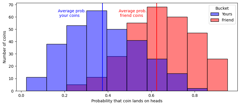
You grab each grab a single coin at random from your containers, and flip them and observe whether they land on heads or tails, the outcomes $x_i^{(y)}$ and $y_i^{(y)}$, respectively. Since the probabilities each coin lands on heads is random here, you can’t actually compare the probabilities. But what you can compare are characteristics about your coins’ and your friend’s coins’ probabilities. You could ask, for instance, whether the average probability that your coins land on heads is less than the average probability that your friend’s coins land on heads. The difference is that we are asking about parameters that underly the random probabilities of the random coins in the experiment, and not about the random probabilities themselves.

Much the same, you could assume that not only are the latent positions for Moors and Moops are different, but these might be random too, just like the probabilities of the coins in the example you just learned about. What we mean when we say that the latent position matrices are random, we mean that the latent positions for each node, the vectors ${\overrightarrow{x}}_i^{(p)}$ and ${\overrightarrow{x}}_i^{(r)}$ for each of the $n$ total nodes, are not necessarily fixed quantities. There might be random variables that underly these too: ${\overrightarrow{\mathbf{x}}}_i^{(p)}$ and ${\overrightarrow{\mathbf{x}}}_i^{(r)}$.

You won’t need to go too in-depth here, but the basic idea is that the latent position vectors for each node, ${\overrightarrow{\mathbf{x}}}_i^{(p)}$ and ${\overrightarrow{\mathbf{x}}}_i^{(r)}$, have underlying parameters as well, just like the random probabilities for your coins and your friend’s coins tended to be around $\frac{3}{8}$ and $\frac{5}{8}$ respectively. All of the characteristics that determine how the Moor or Moop latent position vectors can be realized are governed by functions called the distributions of the latent position vectors. We use the symbol $F^{(p)}$ and $F^{(r)}$, respectively, to denote the distribution of the Moop’s latent position vectors and the Moor’s latent position vectors, respectively. When you ask questions about whether $P^{(p)}$ and $P^{(r)}$ differ, now our question no longer boils down to just checking whether the latent positions themselves are different, but whether the distributions of the latent positions are different.

Like we did before, we will make null and alternative hypotheses for these situations. Your null hypothesis is going to be that $H_0:F^{(p)}=F^{(r)}W$, which means that the distributions of the latent positions are the same (like before, we allow for a possible $W$). The alternative hypothesis is going to be that the latent positions for the Moors and the Moops have a different distribution for any possible rotation, $H_A:F^{(p)}\ne F^{(r)}W$.

The general idea is that we will assume as little as possible about the distributions for the latent positions. Two good ways to do this are using an approach called distance correlation or multiscale generalized correlation (MGC). You can do these very easily using graspologic, through the latent_distribution_test function:

from graspologic.inference import latent_distribution_test

nreps = 1000
approach = 'dcorr'  # the strategy for the latent distribution test
ldt_dcorr = latent_distribution_test(AMoop, AMoor, test=approach, metric="euclidean",
                                     n_bootstraps=nreps)

The relevant things to look at for the latent distribution test are the $p$-value:

print("p-value of H0 against HA: {:.4f}".format(ldt_dcorr[1]))

p-value of H0 against HA: 0.0719

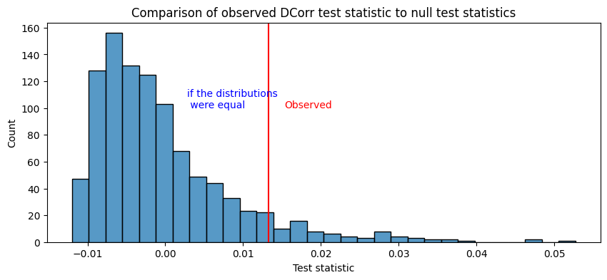
In this case, the distance correlation/MGC approaches produce a test statistic which has a relatively similar interpretation to the one which we used before (the norm of the difference of the estimated latent positions). When these test statistics are relatively large, the two distributions are different. Again, we figure out what we mean by “relative” by using resampling techniques (in this case, non-parametric permutation testing), and we produce estimates of what the test statistic would look like if the distributions were the same and compare to the one we saw in our samples:

Click to show

fig, ax = plt.subplots(1, 1, figsize=(10, 4))
null_distn = DataFrame({"Null dcorrs" : ldt_dcorr[2]["null_distribution"]})
sns.histplot(null_distn, x="Null dcorrs", bins=30, ax=ax)
ax.set_xlabel("Test statistic")
ax.axvline(ldt_dcorr[0], color="red")
ax.text(ldt_dcorr[0] + .002, y=100, color="red", s="Observed")
ax.text(np.quantile(ldt_dcorr[2]["null_distribution"], .75), y=100, color="blue", s="if the distributions\n were equal")
ax.set_title("Comparison of observed DCorr test statistic to null test statistics");

For more details on these approaches, check out [3] and [4].

7.1.4. The Latent distribution test is more conservative than the latent position test

The latent distribution test is called non-parametric because it does not make the assumption that the networks are RDPGs with fixed latent position matrices like we did in the latent position test. In this sense, the latent distribution test tends to be a little bit more general than the latent position test, and will tend to be more conservative. In statistics, we like conservative tests, because it gives us more confidence that our assumptions did not impact our conclusions. When we obtain results in favor of $H_A$ with conservative tests (such as a small $p$-value), we tend to have a little bit more confidence that our results hold up to scrutiny, which is a good thing if you are trying to convince people you are right!

Moreover, the latent position test assumes that the two networks have node matching: node $1$ in the first network has the same interpretation as node $1$ in the second network, and so on for all $n$ nodes in the network. The latent distribution test does not make this rather limiting assumption: you can perform a latent distribution test when the nodes differ in both interpretation (nodes don’t need to be matched) or in number (you could compare networks without the same number of nodes entirely). This makes the latent distribution test a bit more flexible, in general, than the latent position test.

7.1.5. References

The appendix section Section 12.2 discusses the implications of latent distribution testing with respect to spectral embeddings.

1

John C. Gower and Garmt B. Dijksterhuis. Procrustes Problems (Oxford Statistical Science Series, 30). Oxford University Press, Oxford, England, UK, April 2004. ISBN 978-0-19851058-1. URL: https://www.amazon.com/Procrustes-Probn2017ms-Oxford-Statistical-Science/dp/0198510586.

2

Minh Tang, Avanti Athreya, Daniel L. Sussman, Vince Lyzinski, Youngser Park, and Carey E. Priebe. A Semiparametric Two-Sample Hypothesis Testing Problem for Random Graphs. J. Comput. Graph. Stat., 26(2):344–354, April 2017. doi:10.1080/10618600.2016.1193505.

3

Minh Tang, Avanti Athreya, Daniel L. Sussman, Vince Lyzinski, and Carey E. Priebe. A nonparametric two-sample hypothesis testing problem for random graphs. Bernoulli, 23(3):1599–1630, August 2017. doi:10.3150/15-BEJ789.

4

A. Alyakin, Joshua Agterberg, Hayden S. Helm, and C. Priebe. Correcting a Nonparametric Two-sample Graph Hypothesis Test for Graphs with Different Numbers of Vertices. arXiv: Methodology, 2020. URL: https://www.semanticscholar.org/paper/Correcting-a-Nonparametric-Two-sample-Graph-Test-of-Alyakin-Agterberg/c8265eba85e51020be7af24debd467accf2f073b.