9.1. Random walk and diffusion-based methods#

Although this book puts a heavy emphasis on spectral methods, there are many ways in which you can learn lower-dimensional representations for networks which don’t involve spectral approaches. As opposed to spectral methods, a random walk on a network is a random process which focuses on the analysis of paths which start at a node in the network, and proceed to generate successions of random steps to other nodes in the network. The manner in which these random processes materialize is a function of the topology of the random network, including the nodes, edges, and (optionally, if the network is weighted), the edge weights.

9.1.1. A simplified first-order random walk on a network#

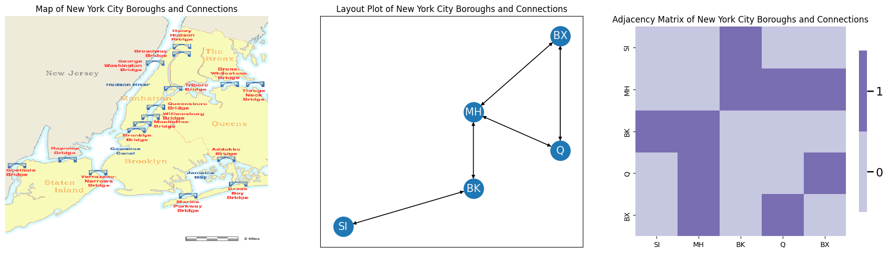
For instance, let’s consider an extremely simplified approach for a first-order random walk on the network that you saw back in Section 3.2, which was our New York example. To begin, let’s redefine the nodes and edges of the network. The nodes of the network are the five boroughs of New York City (Staten Island SI, Brooklyn BK, Queens Q, the Bronx BX, and Manhattan MH). The nodes in your network are the five boroughs. The edges $(i,j)$ of your network exist if one can travel from borough $i$ to borough $j$ along a bridge.

Below, you will look at a map of New York City, with the bridges connecting the different boroughs. In the middle, you look at this map as a network layout plot. The arrows indicate the direction of travel. On the right, you look at this map as an adjacency matrix:

import numpy as np

# define the node names
node_names = np.array(["SI", "MH", "BK", "Q", "BX"])
# define the adjacency matrix
A = np.array([[0,0,1,0,0],  # staten island is neighbors of brooklyn
              [0,0,1,1,1],  # manhattan is neighbors of all but staten island
              [1,1,0,0,0],  # brooklyn is neighbors of staten island and manhattan
              [0,1,0,0,1],  # queens is neighbors of manhattan and bronx
              [0,1,0,1,0]]) # bronx is neighbors of manhattan and queens

import networkx as nx
import matplotlib.pyplot as plt
import matplotlib.image as mpimg
from graphbook_code import heatmap

img = mpimg.imread('../../representations/ch4/img/newyork.png')

G = nx.DiGraph()

G.add_node("SI", pos=(1,1))
G.add_node("MH", pos=(4,4))
G.add_node("BK", pos=(4,2))
G.add_node("Q", pos=(6,3))
G.add_node("BX", pos=(6,6))

pos = nx.get_node_attributes(G, 'pos')
G.add_edge("SI", "BK")
G.add_edge("MH", "BK")
G.add_edge("MH", "Q")
G.add_edge("MH", "BX")
G.add_edge("Q", "BX")

G.add_edge("BK", "SI")
G.add_edge("BK", "MH")
G.add_edge("Q", "MH")
G.add_edge("BX", "MH")
G.add_edge("BX", "Q")

fig, axs = plt.subplots(1,3, figsize=(23, 6))
axs[0].imshow(img, alpha=.8, interpolation='nearest', aspect='auto')
axs[0].axis('off')
axs[0].set_title("Map of New York City Boroughs and Connections")
nx.draw_networkx(G, pos, ax=axs[1], with_labels=True, node_color="tab:blue", node_size = 800,
        font_size=15, font_color="whitesmoke", arrows=True)
axs[1].set_title("Layout Plot of New York City Boroughs and Connections")
heatmap(A, ax=axs[2], xticklabels=[0.5,1.5,2.5,3.5,4.5], yticklabels=[0.5,1.5,2.5,3.5,4.5])
axs[2].set_title("Adjacency Matrix of New York City Boroughs and Connections")
axs[2].set_xticklabels(node_names)
axs[2].set_yticklabels(node_names)
fig;

../../_images/random-walk-diffusion-methods_3_0.png

You are staying at a hotel which is located in Manhattan, and you decide that you are going to explore the city as follows. When you are in a given borough $i$, you will determine the next borough you will explore by letting random chance do the work for you. To better define a first-order random walk, we need to introduce a background concept first: the Markov chain and the Markov property.

9.1.1.1. Markov chains and the markov property#

A finite-space markov chain is a model of a random system in which we have a sequence of possible events which can occur which are finite (the boroughs we will visit on a day $t$) in which the probability of each event depends only on the event in which you were previously. For network analysis, we only need to think about finite-space Markov chains, because the network has a finite collection of possible events which can occur (the nodes in the network being visited). To put this down quantitatively, the markov chain is represented by the sequence $\mathbf s_0, \mathbf s_1, \mathbf s_2, ...$, where each $\mathbf s_t$ takes the value of one of the $n$ total nodes in the network.

You will notice that in our definition of the finite-space markov chain, we made a disclaimer: the probability of each event depends only on the state in which we were previously. This is called the markov property. The idea is that, if we were in Manhattan at the previous step in time $t - 1$ (e.g., $\mathbf s_{t-1}$ realized the value $v_{MH}$, or $\mathbf s_{t-1} = v_{MH}$ for short), that if our current step in the Markov Chain were Brooklyn ($\mathbf s_t = v_{BK}$), that the next step in the Markov chain would not depend at all on the fact that we already saw Manhattan.

9.1.1.1.1. First-order random walks on a network as a markov chain#

To exhibit the ideas of a markov chain, we’ll define a first-order random walk on your New York Boroughs. Remember that the borough you are at, $i$, has $d_i$ possible neighboring boroughs, where $d_i$ was the degree of node $i$. You will visit one of the other nodes in the network as follows. If borough $j$ is a neighbor of borough $i$ (an edge exists from borough $i$ to borough $j$), you will visit borough $j$ with probability $\frac{1}{d_i}$. The idea is that you will visit neighbors of each borough at random, depending only on whether you can get to that borough along an edge of the network. This is called a first-order random walk because it is a random walk where you ignore everything about the path you have taken to get to your current borough to date, except for the fact that you are at that borough now. This means that your next borough will not depend at all on whether you have already been to that borough in your exploration of the city. If the node is not a neighbor of your current borough, you will visit it with probability $0$. Stated another way, if you are in node $i$, the probability of going to another node $j$ is defined as:

\[\begin{align*} p_{ij} &= \begin{cases} \frac{1}{d_i} & \text{edge $(i,j)$ exists} \\ 0 & \text{edge $(i,j)$ does not exist} \end{cases} \end{align*}\]

Note that these probabilities, called the transition probability from node $i$ to node $j$, do not have anything to do with which nodes we have visited yet, and these transition probabilities are always the same! For this reason, they are often organized into a matrix, called the transition probability matrix $P$. In this case, the transition probability matrix looks like this:

# compute the degree of each node
di = A.sum(axis=0)
# the probability matrix is the adjacency divided by
# degree of the starting node
P = (A / di).T

fig, axs = plt.subplots(1,2, figsize=(16, 6))

nx.draw_networkx(G, pos, ax=axs[0], with_labels=True, node_color="tab:blue", node_size = 800,
        font_size=15, font_color="whitesmoke", arrows=True)
axs[0].set_title("Layout Plot of New York City Boroughs and Connections")
heatmap(P, ax=axs[1], xticklabels=[0.5,1.5,2.5,3.5,4.5], yticklabels=[0.5,1.5,2.5,3.5,4.5])
axs[1].set_title("Transition probability matrix $P$ for New York Random Walk")
axs[1].set_xticklabels(["SI", "MH", "BK", "Q", "BX"])
axs[1].set_yticklabels(["SI", "MH", "BK", "Q", "BX"])
axs[1].set_ylabel("Starting borough $i$")
axs[1].set_xlabel("Next borough $j$")
fig;

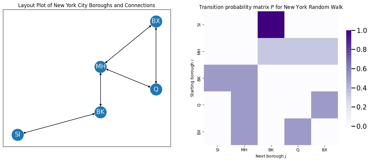
../../_images/random-walk-diffusion-methods_6_0.png

To understand this transition probability matrix, let’s think about the individual rows. Notice that if you are in Staten Island, there is only one borough you can go from here, so with probability $1$, you will visit its only neighbor: Brooklyn. If you are in Manhattan, you could go to any of its three neighbors (Brooklyn, Queens, or Bronx), with equal probability $\frac{1}{3}$. If you were in Brooklyn, you could visit any of its two neighbors (Manhattan or Staten Island) with equal probability $\frac{1}{2}$. This continues for each node in the network until you have successfully generated the transition probability matrix $P$.

There are a lot of interesting properties you can use the transition probability matrix $P$ to learn about, but we won’t cover them all here. If you want some more details on transition probability matrices and Markov chains in general, we would recommend that you check out a book on stochastic processes, such as our favorite [1].

Next, let’s use this transition probability matrix to generate a random walk on the New York City boroughs. As we mentioned, your hotel is in Manhattan, so you are going to start your random walk through the city here. In other words, $\mathbf s_0 = v_{MH}$. For your next step in the Markov chain, you will visit either Brooklyn, Bronx, or Queens with probability $\frac{1}{3}$, or Staten Island with probability $0$. In the following figure, we show the place you start out at, Manhattan, in blue, and the other nodes in gray:

G = nx.DiGraph()

G.add_node("SI", pos=(1,1))
G.add_node("MH", pos=(4,4))
G.add_node("BK", pos=(4,2))
G.add_node("Q", pos=(6,3))
G.add_node("BX", pos=(6,6))

pos = nx.get_node_attributes(G, 'pos')
G.add_edge("SI", "BK")
G.add_edge("MH", "BK")
G.add_edge("MH", "Q")
G.add_edge("MH", "BX")
G.add_edge("Q", "BX")

G.add_edge("BK", "SI")
G.add_edge("BK", "MH")
G.add_edge("Q", "MH")
G.add_edge("BX", "MH")
G.add_edge("BX", "Q")

Ghl = nx.DiGraph()
Ghl.add_node("MH")

fig, ax = plt.subplots(1,1, figsize=(8, 6))
nx.draw_networkx(G, pos, ax=ax, with_labels=True, node_color="tab:gray", node_size = 800,
        font_size=15, font_color="whitesmoke", arrows=True)
nx.draw_networkx(Ghl, pos, ax=ax, with_labels=True, node_color="tab:blue", node_size = 800,
        font_size=15, font_color="whitesmoke", arrows=True)

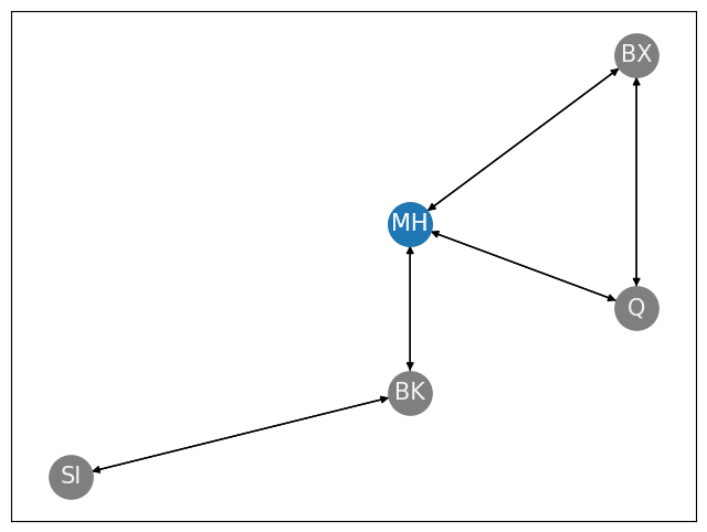
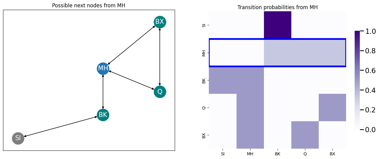
../../_images/random-walk-diffusion-methods_8_0.png

You can visit each of the neighboring nodes, shown in the next plot teal yellow, and the probabilities of visiting each of these nodes are correspondingly highlighted in the transition probability matrix with a blue block:

import matplotlib.patches as patches
Gn = nx.DiGraph()
Gn.add_node("BX")
Gn.add_node("BK")
Gn.add_node("Q")
fig, ax = plt.subplots(1,2, figsize=(16, 6))
nx.draw_networkx(G, pos, ax=ax[0], with_labels=True, node_color="tab:gray", node_size = 800,
        font_size=15, font_color="whitesmoke", arrows=True)
nx.draw_networkx(Ghl, pos, ax=ax[0], with_labels=True, node_color="tab:blue", node_size = 800,
        font_size=15, font_color="whitesmoke", arrows=True)
nx.draw_networkx(Gn, pos, ax=ax[0], with_labels=True, node_color="teal", node_size = 800,
        font_size=15, font_color="whitesmoke", arrows=True)
ax[0].set_title("Possible next nodes from MH")

heatmap(P, ax=ax[1], xticklabels=[0.5,1.5,2.5,3.5,4.5], yticklabels=[0.5,1.5,2.5,3.5,4.5])
ax[1].set_title("Transition probabilities from MH")
ax[1].set_xticklabels(["SI", "MH", "BK", "Q", "BX"])
ax[1].set_yticklabels(["SI", "MH", "BK", "Q", "BX"])

ax[1].add_patch(
     patches.Rectangle(
         (0,1),
         5.0,
         1.0,
         edgecolor='blue',
         fill=False,
         lw=4
     ) )

fig;

../../_images/random-walk-diffusion-methods_10_0.png

You then choose the next node to visit, using these transition probabilities, by generating the probability vector of the next step in the random walk given the current step. We will denote this probability vector with the symbol $\vec p^{(t+1)}_i$, which is the probability vector for which node you will visit at the next step $t+1$ given that you are currently at node $i$. Notice that this is just the entries of the $i^{th}$ row of the transition probability matrix, which can be calculated using the relationship:

\[\begin{align*} \vec p^{(t+1)}_i &= P^\top \vec x^{(i)} \end{align*}\]

where $\vec x^{(i)}$ is the vector which has a value of $0$ for all entries except for entry $i$, where it has a value of $1$. This ends up pulling out the $i^{th}$ row of $P$, because every multiplication except for those against the $i^{th}$ column of $P^\top$ (which is the $i^{th}$ row of $P$, by definition of a transpose) will end up just being $0$! We can see this with the following detailed exploration:

\[\begin{align*} \vec p^{(t+1)}_i &= \begin{bmatrix} p_{11} & ... & p_{1n} \\ \vdots & \ddots & \vdots \\ p_{n1} & ... & p_{nn} \end{bmatrix}^\top\vec x^{(i)} \\ &= \begin{bmatrix} p_{11} & ... & p_{n1} \\ \vdots & \ddots & \vdots \\ p_{1n} & ... & p_{nn} \end{bmatrix}^\top\vec x^{(i)},\;\;\;\;\text{in this step, we just transposed $P$} \\ &= \begin{bmatrix} p_{11}x_{1}^{(i)} + p_{21} x_2^{(i)} + ... p_{n1}x_n^{(i)} \\ \vdots \\ p_{1n}x_{1}^{(i)} + p_{2n} x_2^{(i)} + ... p_{nn}x_n^{(i)} \end{bmatrix},\;\;\;\;\text{the definition of matrix multiplication} \\ &= \begin{bmatrix} p_{i1} \\ \vdots \\ p_{in} \end{bmatrix} \end{align*}\]

where the last step in the multiplication is because $x_{i}^{(i)}$ is the only entry which has a value of $1$, so all of the other multipilications are just $0$. We can pick the next node easily by just using numpy:

xt = np.array([0,1,0,0,0])  # x vector indicating we start at MH
pt2 = P.T @ xt  # p vector for timestep t+1 starting at node MH at time t
# choose the next node using the probability vector we calculated
next_node = np.random.choice(range(0, len(node_names)), p=pt2)
print("Next node: {:s}".format(node_names[next_node]))

Next node: BX

We indicate the path we took between Manhattan and our realized next node in green, shown below:

next_name = node_names[next_node]
Gnext = nx.DiGraph()
Gnext.add_node("MH")
Gnext.add_node(next_name)
Gnext.add_edge("MH", next_name)
fig, ax = plt.subplots(1,1, figsize=(8, 6))
nx.draw_networkx(G, pos, ax=ax, with_labels=True, node_color="tab:gray", node_size = 800,
        font_size=15, font_color="whitesmoke", arrows=True)
nx.draw_networkx(Gnext, pos, ax=ax, with_labels=True, node_color="tab:green", node_size = 800,
        font_size=15, font_color="whitesmoke", arrows=True, edge_color="green", width=4)
nx.draw_networkx(Ghl, pos, ax=ax, with_labels=True, node_color="tab:blue", node_size = 800,
        font_size=15, font_color="whitesmoke", arrows=True)
ax.set_title("1-step of a first-order random walk starting at MH");

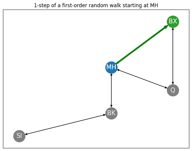
../../_images/random-walk-diffusion-methods_14_0.png

This gives us a realization of $\mathbf s_1$ as the indicated node in the network, conditional on the starting node being $\mathbf s_0 = v_{MH}$. We can generate a $T$-step first-order random walk along the network $G$ using this approach:

Generating a realization of a first-order random walk

Now that we’ve learned how to make a single step in a first-order random walk, we are ready to generate a realization of a first-order random walk. Given a source node $s_0 = i$, a network $G$ with nodes and edges, an in-out parameter $q$, a return parameter $p$, and a number of steps to proceed $T$, we take the following procedure:

Generate the first-order transition probability matrix, $P$, using the adjacency matrix of the network, $A$.
For $t = 1:T$:
- choose the next node to visit $s_{t}$, by selecting a node $j$ with probability $p_{s_tj}$.

The sequence $\{s_0, s_1, ..., s_T\}$ is a realization of a $T$-step first-order random walk along the network $G$.

9.1.2. What do markov chains and random walks have to do with embedding networks?#

In the preface for this section, we said we were going to cover how to use a random walk to embed our network, but we’ve ignored that thus far! To get us to what this has to do with embeddings, we need to introduce a slight variation of the random walk we developed in the preceding section, called the second-order biased random walk.

9.1.2.1. Second-order biased random walk#

Remember when we developed our first-order random walk, we did something kind of nonsensical: we ignored all of the previous boroughs of New York you had already seen, and said that the next borough was only a function of the current borough you are at. You could certainly imagine that you get caught in a legitimate random walk (it is a possible realization because all of the transition probabilities are positive) where you explore going from Manhattan to Brooklyn, and then over to Staten Island, and then back to Brooklyn, and then back to Staten Island, so on and so forth, because you totally ignored the previous places you had been when making your decision for where to go from your current borough.

If you are a tourist trying to explore New York, you obviously will want to get a better sense of all of the city, and want to favor the boroughs you haven’t been to as recently! In the second-order biased random walk, we introduce the idea of the return and in-out parameters, $p$ and $q$, respectively.

9.1.2.1.1. The bias factor lets us control our ability to leave or remain amongst a neighborhood of nodes#

Remember that the steps in our random walk, $\left\{\mathbf s_0, \mathbf s_1, ..., \mathbf s_{t-1}, \mathbf s_t, ...\right\}$, were sequences of random variables which took values of our nodes in the network. Let’s assume that we have a random walk so far, where at our previous state, $\mathbf s_{t-1} = s_{t-1}$, and we are currently at node $i$, $\mathbf s_t = i$. Here, $s_{t-1}$ is some other node which we just came from to get to node $i$.

The in-out parameter $q$ is a value which indicates a bias factor of $\frac{1}{q}$ that we will go to some node $j$ that is totally disconnected from the previous node that we visited, $s_{t-1}$. This means that in our network, there is no edge starting at node $j$ and going to node $s_{t-1}$. If the in-out parameter $q$ takes big values, then $\frac{1}{q}$ will be very small, and we will be biased against visiting nodes which are not connected to the previous node we visited. If $q$ is small, then $\frac{1}{q}$ will be very big, and we will be biased towards visiting nodes which are not connected to the previous node we visited.

The return parameter $p$ is a value which indicates a bias factor of $\frac{1}{p}$ that we will go back to the node which we visited previously in the last state $s_{t-1}$. If the return parameter $p$ takes big values, $\frac{1}{p}$ will be very small, and we will be biased against visiting a node we have just been to. If $p$ is small, then $\frac{1}{p}$ will be very big, and we will be biased towards visiting a node which we were just at.

If a node satisfies neither of these conditions, the bias factor is just left at $1$. Together, these relationships are summarized with the bias factor $\alpha_{ij}^{(t+1)}(p,q, s_{t-1})$ starting at node $i$ and proceeding to node $j$ with parameters $p$ and $q$ for the next step $t+1$ given that we just left state $s_{t-1}$ as:

\[\begin{align*} \alpha_{ij}(p,q,s_{t-1}) &= \begin{cases} \frac{1}{p} & \text{$s_{t-1} = j$} \\ \frac{1}{q} & \text{$s_{t-1} \neq j$ and the edge $(j,s_{t-1})$ exists} \\ 1 & \text{$s_{t-1} \neq j$ and no edge $(j,s_{t-1})$ exists} \end{cases} \end{align*}\]

And the corresponding bias vector $\vec \alpha_i(p,q, s_{t-1})$, which is a vector of each of the bias factors for all of the $n$ nodes in the network (which are indexed by $j$).

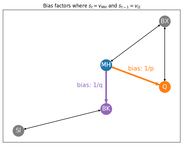
Let’s use our New York example to get a sense of how these bias vectors work. We’ll consider a random walk at some arbitrary current state $t$, where the current node we are on is Manhattan ($s_t = v_{MH}$) and is shown in blue, and the previous node we visited was Queens ($s_{t-1} = v_{Q}$) and is shown in orange. We just visited node $Q$, so the bias factor will be $\frac{1}{p}$ (the edge is shown in orange). The node for Bronx has an edge back to Queens, so the bias factor will be $\frac{1}{q}$ (the edge is shown in purple). The node for Brooklyn does not have an edge back to queens, so the bias is $1$ (and the edge is shown in black):

fig, ax = plt.subplots(1,1, figsize=(8, 6))
nx.draw_networkx(G, pos, ax=ax, with_labels=True, node_color="tab:gray", node_size = 800,
                 font_size=15, font_color="whitesmoke", arrows=True)
ax.set_title("Bias factors where $s_t = v_{MH}$ and $s_{t-1} = v_{Q}$")

nx.draw_networkx(Ghl, pos, ax=ax, with_labels=True, node_color="tab:blue", node_size = 800,
                 font_size=15, font_color="whitesmoke", arrows=True)
Gin = nx.DiGraph()
Gin.add_node("BK", pos=(1,1))
Gin.add_node("MH", pos=(4,4))
Gin.add_edge("MH", "BK")

nx.draw_networkx(Gin, pos, ax=ax, with_labels=True, node_color="tab:purple", node_size = 800,
                 font_size=15, font_color="whitesmoke", arrows=True, edge_color="tab:purple",
                 width=4)
Gret = nx.DiGraph()
Gret.add_node("Q")
Gret.add_node("MH")
Gret.add_edge("MH", "Q")

nx.draw_networkx(Gret, pos, ax=ax, with_labels=True, node_color="tab:orange", node_size = 800,
                 font_size=15, font_color="whitesmoke", arrows=True, edge_color="tab:orange",
                 width=4)
nx.draw_networkx(Ghl, pos, ax=ax, with_labels=True, node_color="tab:blue", node_size = 800,
                 font_size=15, font_color="whitesmoke", arrows=True)
ax.annotate("bias: 1/p", (4.75, 3.75), size=15, color="tab:orange")
ax.annotate("bias: 1/q", (3, 3), size=15, color="tab:purple");

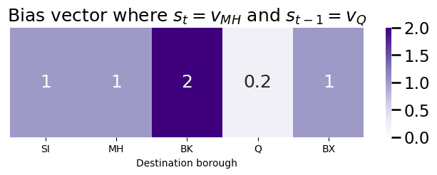
../../_images/random-walk-diffusion-methods_18_0.png

If we were to tend to bias against returning (a large return parameter, say $p = 5$) and towards in-out (a small in-out parameter, say $q = \frac{1}{2}$), the bias vector will look like this:

p = 5  # return parameter
q = 1/2  # in-out parameter
bias_vector = np.ones(len(node_names))
bias_vector[node_names == "Q"] = 1/p
bias_vector[node_names == "BK"] = 1/q

import seaborn as sns

def plot_vec(vec, title="", blockname="Destination borough", 
             blocklabs=node_names,
             blocktix=[0.5 + i for i in range(0, len(node_names))],
             vmax=None, ax=None, cbar=True, cbar_ax=None):
    if ax is None:
        fig, ax = plt.subplots(figsize=(8, 2))
    
    if vmax is None:
        vmax = vec.max()
    with sns.plotting_context("talk", font_scale=1):
        if cbar_ax is not None:
            ax = sns.heatmap(vec.reshape((1,vec.shape[0])), cbar=cbar, cbar_ax=cbar_ax, cmap="Purples",
                            ax=ax, cbar_kws=dict(shrink=1), yticklabels=False,
                            xticklabels=False, vmin=0, vmax=vmax, annot=True)
        else:
            ax = sns.heatmap(vec.reshape((1,vec.shape[0])), cbar=cbar, cmap="Purples",
                            ax=ax, cbar_kws=dict(shrink=1), yticklabels=False,
                            xticklabels=False, vmin=0, vmax=vmax, annot=True)
        ax.set_title(title)
        ax.set(xlabel=blockname)
        ax.set_xticks(blocktix)
        ax.set_xticklabels(blocklabs)
        if cbar_ax is None and cbar:
            cbar = ax.collections[0].colorbar
            cbar.ax.set_frame_on(True)
    return

plot_vec(bias_vector, title="Bias vector where $s_t = v_{MH}$ and $s_{t-1} = v_{Q}$")

../../_images/random-walk-diffusion-methods_21_0.png

9.1.2.1.2. Adjusting the transition probabilities with the bias vector#

In our second order random walk, instead of the transition probabilities being a function only of the current state, they are also a function of the preceding state we were at $s_{t-1}$. This means that our transition probability matrix is going to look different based on which node we just came from. The transition probabilities are defined using the indexed triplet $p_{s_{t-1}ij}(p,q)$, where $s_{t-1}$ is the preceding node we visited, $i$ is the current node we are at, $j$ is any other node in the network, and $p$ and $q$ are the return and in-out parameters respectively. The second-order biased transition factors the terms:

\[\begin{align*} \beta_{s_{t-1}ij}(p,q) &= \alpha_{ij}(p, q, s_{t-1})p_{ij} \end{align*}\]

where $p_{ij}$ are the first-order markov transition probabilities we used previously. These are called second-order because they depend on the current node, $i$, as well as the preceding node, $s_{t-1}$.

In effect, what this statement says is that all we do is up or down-weight (or don’t change it at all, if the bias factor is $1$) the probability $p_{ij}$ of going from node $i$ to node $j$ based on the bias factor $\alpha_{ij}(p, q, s_{t-1})$. These are no longer probabilities, because starting at a node $i$, we might end up with the bias-adjusted transition factors no longer summing to one. This is because we did not require anything about how $\alpha_{ij}^{(t+1)}(p,q,s_{t-1})$ behaved across all possible nodes $j$ we could transition to from our current node $i$.

Finally, we then use the biased transition factors to compute the second-order biased transition probabilities. These are just normalized versions of the biased transition factors, where we normalize to make sure that they all sum up to one (and hence, produce a valid transition probability from node $i$ outwards):

\[\begin{align*} p_{s_{t-1}ij}(p,q) &= \frac{\beta_{s_{t-1}ij}(p,q)}{\sum_{j' = 1}^n\beta_{s_{t-1}ij'}(p,q)} \end{align*}\]

Notice that in the denominator, that we are just normalizing the bias-adjusted transition factor by the sum of all the other bias-adjusted transition factors from node $i$ to any other nodes $j'$ in the network.

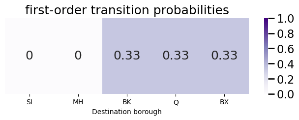
Next, we show how this computation works to update the transition probability vector from the Manhattan node to node $j$ given a previous node of Queens. We begin by first starting with the first-order transition probability vector $\vec p_i$:

xstart = [0, 1, 0, 0, 0]  # starting vector at MH
pvec = P.T @ xstart  # probability vector is Pt*x

plot_vec(pvec, title="first-order transition probabilities", vmax=1)

../../_images/random-walk-diffusion-methods_24_0.png

Next, we compute the bias vector, exactly as we did previously:

plot_vec(bias_vector, title="Bias vector where $s_t = v_{MH}$ and $s_{t-1} = v_{Q}$")

../../_images/random-walk-diffusion-methods_26_0.png

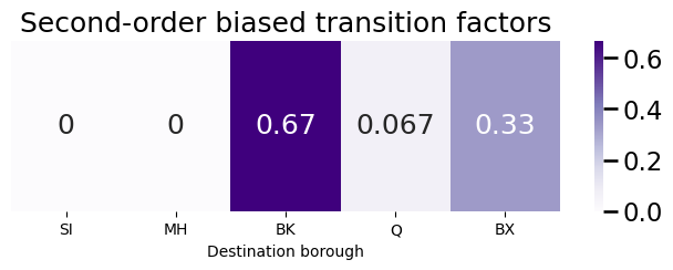
The next step is to compute the second-order biased transition factors:

bias_factors = pvec*bias_vector

plot_vec(bias_factors, title="Second-order biased transition factors")

../../_images/random-walk-diffusion-methods_29_0.png

And finally, to normalize the bias-adjusted transition factors to obtain the second-order biased transition probabilities. We compare the second-order biased transition probabilities to the first-order transition probabilities, so that you can see the impact that the second-order biasing procedure had on our probability vector:

biased_pvec = bias_factors/bias_factors.sum()

import warnings
warnings.filterwarnings("ignore")

fig, axs = plt.subplots(2, 1, figsize=(8, 4))
cbar_ax = fig.add_axes([.91, .3, .03, .4])

prob_vecs = [pvec, biased_pvec, biased_pvec]
titles = ["first-order transition probs.", "Second-order biased transition probs."]
for i, ax in enumerate(axs.flat):
    plot_vec(prob_vecs[i], ax=ax, vmax=1, cbar=i==2, 
             cbar_ax= cbar_ax if i == 2 else None, title=titles[i])
i=2
plot_vec(biased_pvec, ax=axs[1], vmax=1, cbar=i==2, 
             cbar_ax= cbar_ax, title="Second-order biased transition probs.")
    
fig.tight_layout(rect=[0, 0, .85, 1])

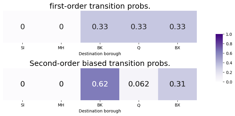
../../_images/random-walk-diffusion-methods_32_0.png

As we can see, our tendency to return to Queens (since we were just there in the previous step, $s_{t-1} = v_{Q}$) has decreased from the first-order transition probability to the second-order biased transition probability, due to the fact that the return parameter is big ($p = 5$). Further, our tendency to move in-out to Brooklyn (since Brooklyn has no edges to Queens) has increased from the first-order transition probability to the second-order biased transition probability, due to the fact that the in-out parameter is small ($q = 0.2$). The transition probability for the remaining nodes, such as BX, with a bias of $1$ are less affected from the first-order to the second-order biased transition probability. We then just use the second-order biased transition probabilities to decide where to go next, and we take that step, shown in green:

xt = np.array([0,1,0,0,0])  # x vector indicating we start at MH
# choose the next node using the second-order biased transition probability
next_node = np.random.choice(range(0, len(node_names)), p=biased_pvec)
print("Next node: {:s}".format(node_names[next_node]))

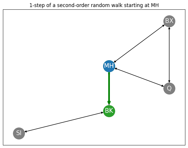
Next node: BK

next_name = node_names[next_node]
Gnext = nx.DiGraph()
Gnext.add_node("MH")
Gnext.add_node(next_name)
Gnext.add_edge("MH", next_name)
fig, ax = plt.subplots(1,1, figsize=(8, 6))
nx.draw_networkx(G, pos, ax=ax, with_labels=True, node_color="tab:gray", node_size = 800,
        font_size=15, font_color="whitesmoke", arrows=True)
nx.draw_networkx(Gnext, pos, ax=ax, with_labels=True, node_color="tab:green", node_size = 800,
        font_size=15, font_color="whitesmoke", arrows=True, edge_color="green", width=4)
nx.draw_networkx(Ghl, pos, ax=ax, with_labels=True, node_color="tab:blue", node_size = 800,
        font_size=15, font_color="whitesmoke", arrows=True)
ax.set_title("1-step of a second-order random walk starting at MH");

../../_images/random-walk-diffusion-methods_35_0.png

Generating a realization of a second-order biased random walk

Now that we’ve learned how to make a single step in a second-order biased random walk, we are ready to generate a realization of a second-order biased random walk. Given a source node $s_0 = i$, a network $G$ with nodes and edges, an in-out parameter $q$, a return parameter $p$, and a number of steps to proceed $T$, we take the following procedure:

Generate the first-order transition probability matrix, $P$, using the adjacency matrix of the network, $A$.
Perform a first-order random walk from the source node $i$ to the first step in our random walk, $s_1 = i'$.
For $t = 2:T$:
- compute the bias from $s_{t-1}$ to all of the other nodes $j$ in the network given that the preceding node was $s_{t-2}$, $\alpha_{s_{t-2}s_{t-1}j}(p,q)$.
- using the bias $\vec\alpha_{s_{t-2}s_{t-1}j}(p,q)$ and the first-order transition probability $p_{s_{t-1}j}$, compute the second-order bias factor $\beta_{s_{t-2}s_{t-1}j}(p,q)$ for each node $j$ in the network.
- normalize the second-order bias factors $\beta_{s_{t-2}s_{t-1}j}(p,q)$ to obtain the second-order transition probabilities $p_{s_{t-2}s_{t-1}j}(p,q)$.
- choose the next node to visit $s_t$, by selecting node $j$ with probability $p_{s_{t-2}s_{t-1}j}(p,q)$.

The sequence $\{s_0, s_1, ..., s_T\}$ is a realization of a $T$-step second-order biased random walk along the network $G$ with parameters $(p,q)$.

9.1.3. node2vec embedding#

Now that we know about second-order biased random walks, we are ready to approach our problem at hand: leveraging random walks to produce structured embeddings. We have one final ingredient to embed our networks: the word2vec algorithm.

9.1.3.1. Word2vec#

The word2vec algorithm is a technique for natural language processing (NLP) developed in 2013 by a team of researchers at Google led by Tomas Mikolov. The algorithm takes in large collections of text data, called a corpus. The algorithm takes this corpus of text along with a desired number of embedding dimensions $d$, and embeds every possible word in the corpus into a $d$-dimensional space such that the contexts of the words frequently used together are preserved. In this case, a context refers to words which tend to convey similar meaning (they are synonyms), words which tend to precede be used together (for instance, “learning” and “intelligence”), and many other attributes of the words. When we say “preserved”, what we mean is that words that have similar contexts tend to be closer together in the embedded space. This embedding can then be used for many things, such as guessing the synonyms of words, suggesting next words for a sentence, and many other things.

We won’t go into too many details here, because the procedure for word2vec requires some heavy background in neural networks which we’ll learn in a much more general context about in the section when we cover Graph Neural Networks in Section 9.2. If you want to learn more about word2vec, we would suggest you dig up some blog posts on sites like medium, or by checking out the original papers by Mikolov and his team, of which the first can be found at [2] and the second can be found [3].

9.1.3.2. Using node2vec to embed the network#

To begin the node2vec procedure, we take our collection of nodes and the desired number of embedding dimensions $d$. Then, for each node, we generate a random walk of length $T$ using the given node as the starting node with parameters $(p,q)$, as we did above. This gives us a collection of random walks with disparate starting nodes in the network. We repeat this procedure a number of times for each possible starting node. Next, we “pretend” that node names are words, and we simply feed the collections of random walks we generated into word2vec algorithm as our “corpus” of text along with the desired number of embedding dimensions $d$. This produces for us a structured $d$-dimensional embedding of each node in the network. Nodes which tend to be along random walks together tend to end up closer in the embedding space, and nodes which do not tend to be along random walks together tend to end up further in the embedding space.

Let’s try embedding an SBM using node2vec. We’re going to leave the in-out and return parameters both equal to one, for now; e.g., $p = q = 1$. We will generate $20$ random walks starting at each node ($w = 20$), and each walk will have a length of $200$ steps ($T = 200$), and we show the probability matrix on the left with a realization on the right:

import graspologic as gp

n1 = 50; n2 = 50
Baff = [[0.5, 0.2], [0.2, 0.5]]

zvecaff = np.array(["C1" for i in range(0, n1)] + ["C2" for i in range(0, n2)])

# the probability matrix
zvecaff_ohe = np.vstack([[1, 0] for i in range(0, n1)] + [[0, 1] for i in range(0, n2)])
Paff = zvecaff_ohe @ Baff @ zvecaff_ohe.T

np1 = 15; nc = 70; np2 = 15
Bcp = [[0.1, 0.1, 0.1],
      [0.1, 0.7, 0.1],
      [0.1, 0.1, 0.1]]


zveccp = np.array(["Per." for i in range(0, np1)] +
                  ["Core" for i in range(0, nc)] +
                  ["Per." for i in range(0, np2)])

# the probability matrix
zveccp_ohe = np.vstack([[1, 0, 0] for i in range(0, np1)] + 
                       [[0, 1, 0] for i in range(0, nc)] +
                       [[0, 0, 1] for i in range(0, np2)])
Pcp = zveccp_ohe @ Bcp @ zveccp_ohe.T

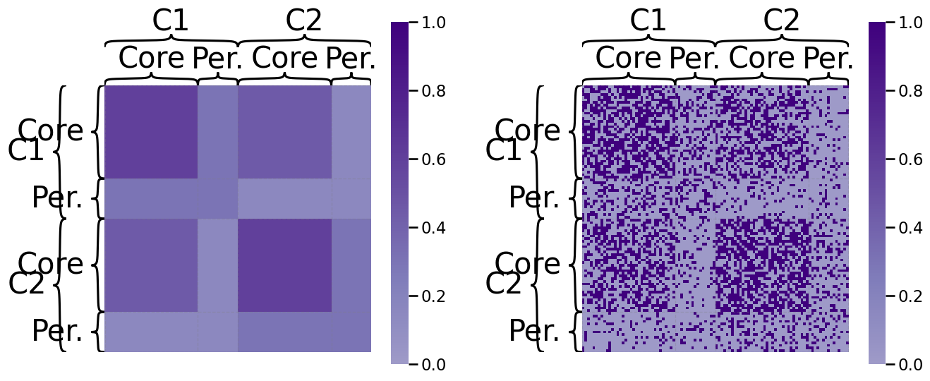
P_aff_and_cp = (Pcp + Paff)/2
np.random.seed(1234)
A_aff_and_cp =  gp.simulations.sample_edges(P_aff_and_cp, directed=False, loops=False)

from graphbook_code import cmaps

fig, axs = plt.subplots(1,2, figsize=(16,9))

gp.plot.heatmap(P_aff_and_cp, ax=axs[0], inner_hier_labels=zveccp, outer_hier_labels=zvecaff,
                title="", vmin=0, vmax=1, cmap=cmaps["sequential"]);
gp.plot.heatmap(A_aff_and_cp, ax=axs[1], inner_hier_labels=zveccp, outer_hier_labels=zvecaff,
                title="", vmin=0, vmax=1, cmap=cmaps["sequential"]);

../../_images/random-walk-diffusion-methods_38_0.png

The resulting embedding produces node embedding vectors which are organized like this, viewed from a pairs plot:

from graspologic.embed import node2vec_embed as node2vec

p = 1; q = 1; w = 20; T = 200
d = 4  # number of embedding dimensions to use
Xhat, _ = node2vec(nx.from_numpy_matrix(A_aff_and_cp), return_hyperparameter=float(p),
                     inout_hyperparameter=float(q), dimensions=d, num_walks=w, walk_length=T,
                     iterations=100)

from graspologic.plot import pairplot

_ = pairplot(Xhat, labels=zvecaff, legend_name="Community")

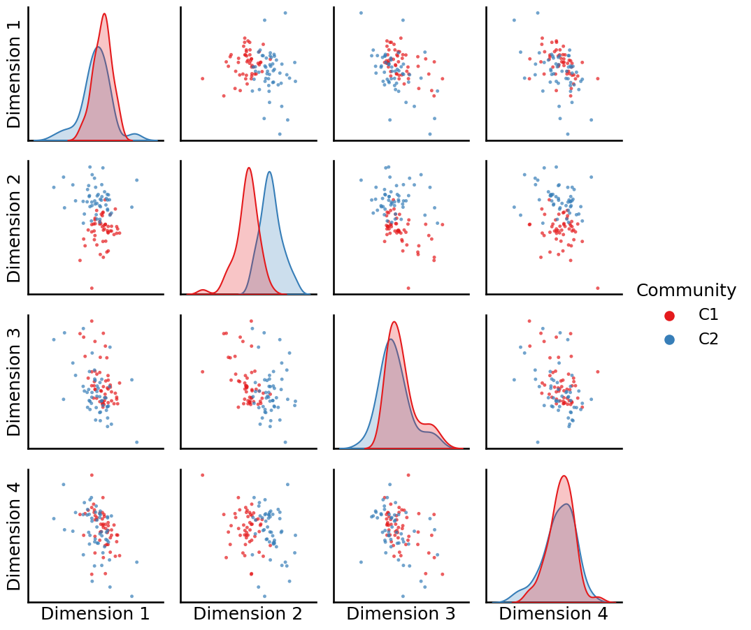
../../_images/random-walk-diffusion-methods_41_0.png

Looking at this pairs plot, we can see that the disparity between communities one and two is largely captured by the first embedding dimension.

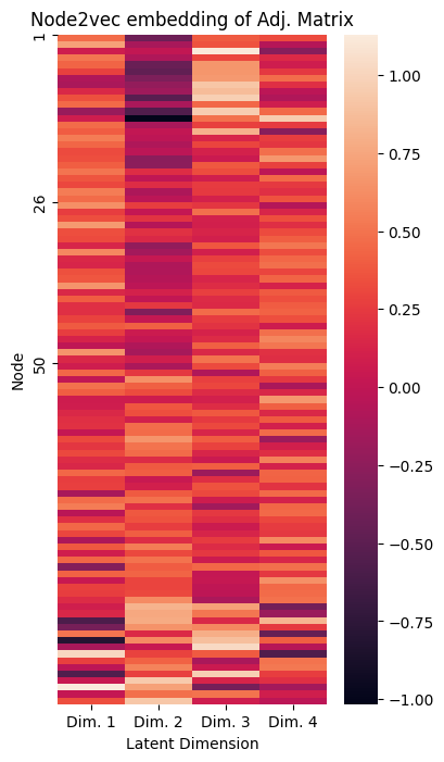
We can also look at this embedding using a heatmap of the individual nodes in the network, like we did for ASE and LSE:

def plot_lpm(D, ax=None, title="", xticks=[], xticklabs=[],
            yticks=[], yticklabs=[], cbar=True):
    if ax is None:
        fig, ax = plt.subplots(1,1, figsize=(3,8))
    sns.heatmap(D, ax=ax, cbar=cbar)
    ax.set_xlabel("Latent Dimension")
    ax.set_ylabel("Node")
    ax.set_xticks(xticks)
    ax.set_xticklabels(xticklabs)
    ax.set_yticks(yticks)
    ax.set_yticklabels(yticklabs)
    ax.set_title(title);

fig, ax = plt.subplots(1, 1, figsize=(4, 8))

plot_lpm(Xhat, xticks=[0.5, 1.5, 2.5, 3.5], ax=ax, title="Node2vec embedding of Adj. Matrix",
         xticklabs=["Dim. 1", "Dim. 2", "Dim. 3", "Dim. 4"], yticks=[0, 25, 49], yticklabs=["1", "26", "50"])

../../_images/random-walk-diffusion-methods_43_0.png

9.1.3.3. Why do we need a second-order biased random walk to generate an embedding?#

You will notice that if we set $p=q=1$, the first-order random walk and the second-order biased random walk turn out to be identical. This is because the biases all turn out to be one, so the “bias factors” turn out to really just be the first-order transition probabilities from the normal random walk. So why do we want the flexibility of the second-order biased random walk, if we can embed our network using the first-order random walk?

The reason is that the second-order biased random walk gives us flexibility. You will notice that since the node2vec procedure relies on the “corpus” of random walks, that the behavior of these random walks will have a substantial influence on the resulting embedding. Let’s see what happens to our embeddings as we tend to favor moving within the same nodes for our random walks more, which means punishing in-out movements ($q$ is larger, so let’s use $q=5$) and up-weighting return movements ($p$ is smaller, so let’s use $p = 0.2$):

p = 0.1; q = 10
d = 4  # number of embedding dimensions to use
Xhat, _ = node2vec(nx.from_numpy_matrix(A_aff_and_cp), return_hyperparameter=float(p),
                     inout_hyperparameter=float(q), dimensions=d, num_walks=w, walk_length=T,
                     iterations=100, random_seed=100)

_ = pairplot(Xhat, labels=zvecaff, legend_name="Community")

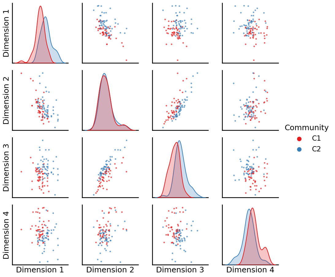
../../_images/random-walk-diffusion-methods_46_0.png

It looks like dimensions one and two do a great job of capturing the differences between the two communities.

Simultaneously, when we remember that the node2vec algorithm builds off the idea of the word2vec algorithm at preserving nodes which have a similar context, we know that the core nodes all share a similar context (they are more strongly connected) than the peripheral nodes (which are less strongly connected). When we plot which nodes are core and which are periphery, we see that:

_ = pairplot(Xhat, labels=zveccp, legend_name="Node type")

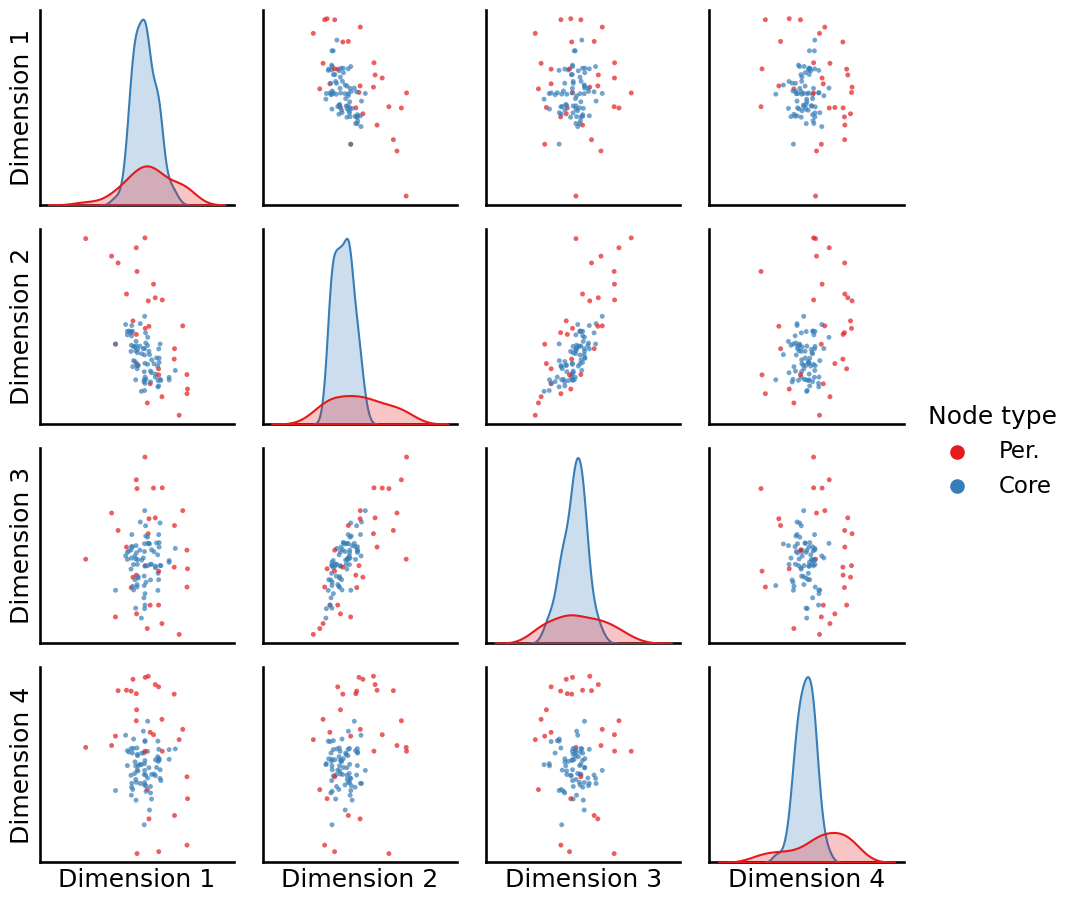
../../_images/random-walk-diffusion-methods_48_0.png

The core nodes (in blue) all tend to be relatively tightly clustered around the around the center across all of the dimensions, and the periphery nodes (in red) tend to be on the exterior of the blob of data. If we have a clustering technique could determine which nodes were in the center versus which nodes were in the exterior, we could effectively capture the core versus the periphery nodes.

Toying around further with these different parameters can yield us very different ways to represent the same network in Euclidean space, and unlike spectral methods, random-walk based methods can preserve numerous desirable properties of our network such as affinity and core-periphery concurrently.

9.1.4. Extending to weighted and directed networks#

It is extremely easy to adapt the strategies we have developed so far to weighted or directed networks. If your network takes non-negative weights, and the weights $w_{ij}$ can be interpreted to indicate the “strength” of a connection between a node $i$ and $j$, you can just let the transition probabilities $p_{ij}$ be the weights normalized by the out-degree from node $i$; that is:

\[\begin{align*} p_{ij} &= \frac{w_{ij}}{d_i} \end{align*}\]

where the out-degree is the quantity $d_i = \sum_{j = 1}^n w_{ij}$.

9.1.5. References#

1: Dean L. Isaacson and Richard W. Madsen. Markov Chains: Theory and Applications. Wiley, Hoboken, NJ, USA, March 1976. ISBN 978-0-47142862-6. URL: https://www.amazon.com/Markov-Chains-Applications-Dean-Isaacson/dp/0471428620.
2: Tomas Mikolov, Kai Chen, Greg Corrado, and Jeffrey Dean. Efficient Estimation of Word Representations in Vector Space. arXiv, January 2013. arXiv:1301.3781, doi:10.48550/arXiv.1301.3781.
3: Tomas Mikolov, Ilya Sutskever, Kai Chen, Greg Corrado, and Jeffrey Dean. Distributed Representations of Words and Phrases and their Compositionality. arXiv, October 2013. arXiv:1310.4546, doi:10.48550/arXiv.1310.4546.

Hands-on Network Machine Learning with Scikit-Learn and Graspologic

Random walk and diffusion-based methods

Contents