11.5. Stochastic Block Models

11.5.1. A Priori Stochastic Block Model

The a priori SBM is an SBM in which we know ahead of time (a priori) which nodes are in which communities. Here, we will use the variable $K$ to denote the maximum number of different communities. The ordering of the communities does not matter; the community we call $1$ versus $2$ versus $K$ is largely a symbolic distinction (the only thing that matters is that they are different). The a priori SBM has the following parameter:

Parameter	Space	Description
$B$	[0,1]${}^{K\times K}$	The block matrix, which assigns edge probabilities for pairs of communities

To describe the A Priori SBM, we will designate the community each node is a part of using a vector, which has a single community assignment for each node in the network. We will call this node assignment vector $\overrightarrow{\tau }$, and it is a $n$-length vector (one element for each node) with elements which can take values from $1$ to $K$. In symbols, we would say that $\overrightarrow{\tau }\in \{1,...,K{\}}^n$. What this means is that for a given element of $\overrightarrow{\tau }$, ${\tau }_i$, that ${\tau }_i$ is the community assignment (either $1$, $2$, so on and so forth up to $K$) for the $i^{th}$ node. If there we hahd an example where there were $2$ communities ($K=2$) for instance, and the first two nodes are in community $1$ and the second two in community $2$, then $\overrightarrow{\tau }$ would be a vector which looks like:

$$\begin{array}{rl}\overrightarrow{\tau }& ={\left[\begin{array}{cccc}1& 1& 2& 2\end{array}\right]}^{\mathrm{\top }}\end{array}$$

Next, let’s discuss the matrix $B$, which is known as the block matrix of the SBM. We write down that $B\in [0,1{]}^{K\times K}$, which means that the block matrix is a matrix with $K$ rows and $K$ columns. If we have a pair of nodes and know which of the $K$ communities each node is from, the block matrix tells us the probability that those two nodes are connected. If our networks are simple, the matrix $B$ is also symmetric, which means that if $b_{k{k}^{\prime }}=p$ where $p$ is a probability, that $b_{k^{\prime }k}=p$, too. The requirement of $B$ to be symmetric exists only if we are dealing with undirected networks.

Finally, let’s think about how to write down the generative model for the a priori SBM. Intuitionally what we want to reflect is, if we know that node $i$ is in community $k^{\prime }$ and node $j$ is in community $k$, that the $(k^{\prime },k)$ entry of the block matrix is the probability that $i$ and $j$ are connected. We say that given ${\tau }_i=k^{\prime }$ and ${\tau }_j=k$, ${\mathbf{a}}_{ij}$ is sampled independently from a $Bern(b_{k^{\prime }k})$ distribution for all $j>i$. Note that the adjacencies ${\mathbf{a}}_{ij}$ are not necessarily identically distributed, because the probability depends on the community of edge $(i,j)$. If $\mathbf{A}$ is an a priori SBM network with parameter $B$, and $\overrightarrow{\tau }$ is a realization of the node-assignment vector, we write that $\mathbf{A}\sim SB{M}_{n,\overrightarrow{\tau }}(B)$.

11.5.1.1. Probability

What does the probability for the a priori SBM look like? In our previous description, we admittedly simplified things to an extent to keep the wording down. In truth, we model the a priori SBM using a latent variable model, which means that the node assignment vector, $\overrightarrow{\tau \tau }$, is treated as random. For the case of the a priori SBM, it just so happens that we know the specific value that this latent variable $\overrightarrow{\tau \tau }$ takes, $\overrightarrow{\tau }$, ahead of time.

Fortunately, since $\overrightarrow{\tau }$ is a parameter of the a priori SBM, the probability is a bit simpler than for the a posteriori SBM. This is because the a posteriori SBM requires an integration over potential realizations of $\overrightarrow{\tau \tau }$, whereas the a priori SBM does not, since we already know that $\overrightarrow{\tau \tau }$ was realized as $\overrightarrow{\tau }$.

Putting these steps together gives us that:

$$\begin{array}{rl}P{r}_{\theta }(A)& =P{r}_{\theta }(\mathbf{A}=A|\overrightarrow{\tau \tau }=\overrightarrow{\tau })\\ & =\prod _{j>i}P{r}_{\theta }({\mathbf{a}}_{ij}=a_{ij}|\overrightarrow{\tau \tau }=\overrightarrow{\tau }),\text{Independence Assumption}\end{array}$$

Next, for the a priori SBM, we know that each edge ${\mathbf{a}}_{ij}$ only actually depends on the community assignments of nodes $i$ and $j$, so we know that $P{r}_{\theta }({\mathbf{a}}_{ij}=a_{ij}|\overrightarrow{\tau \tau }=\overrightarrow{\tau })=Pr({\mathbf{a}}_{ij}=a_{ij}|{\tau }_i=k^{\prime },{\tau }_j=k)$, where $k$ and $k^{\prime }$ are any of the $K$ possible communities. This is because the community assignments of nodes that are not nodes $i$ and $j$ do not matter for edge $ij$, due to the independence assumption.

Next, let’s think about the probability matrix $P=(p_{ij})$ for the a priori SBM. We know that, given that ${\tau }_i=k^{\prime }$ and ${\tau }_j=k$, each adjacency ${\mathbf{a}}_{ij}$ is sampled independently and identically from a $Bern(b_{k^{\prime },k})$ distribution. This means that $p_{ij}=b_{k^{\prime },k}$. Completing our analysis from above:

$$\begin{array}{rl}P{r}_{\theta }(A)& =\prod _{j>i}{b}_{k^{\prime }k}^{a_{ij}}(1-b_{k^{\prime }k}{)}^{1-a_{ij}}\\ & =\prod _{k,k^{\prime }\in [K]}{b}_{k^{\prime }k}^{m_{k^{\prime }k}}(1-b_{k^{\prime }k}{)}^{n_{k^{\prime }k}-m_{k^{\prime }k}}\end{array}$$

Where $n_{k^{\prime }k}$ denotes the total number of edges possible between nodes assigned to community $k^{\prime }$ and nodes assigned to community $k$. That is, $n_{k^{\prime }k}=\sum _{j>i}{\mathbb{1}}_{{\tau }_i=k^{\prime }}{\mathbb{1}}_{{\tau }_j=k}$. Further, we will use $m_{k^{\prime }k}$ to denote the total number of edges observed between these two communities. That is, $m_{k^{\prime }k}=\sum _{j>i}{\mathbb{1}}_{{\tau }_i=k^{\prime }}{\mathbb{1}}_{{\tau }_j=k}{a}_{ij}$. Note that for a single $(k^{\prime },k)$ community pair, that the probability is analogous to the probability of a realization of an ER random variable.

Like the ER model, there are again equivalence classes of the sample space ${\mathcal{A}}_n$ in terms of their probability. For a two-community setting, with $\overrightarrow{\tau }$ and $B$ given, the equivalence classes are the sets:

$$\begin{array}{rl}{E}_{a,b,c}(\overrightarrow{\tau },B)& =\{A\in {\mathcal{A}}_n:m_{11}=a,m_{21}=m_{12}=b,m_{22}=c\}\end{array}$$

The number of equivalence classes possible scales with the number of communities, and the manner in which nodes are assigned to communities (particularly, the number of nodes in each community).

11.5.2. A Posteriori Stochastic Block Model

In the a posteriori Stochastic Block Model (SBM), we consider that node assignment to one of $K$ communities is a random variable, that we don’t know already like te a priori SBM. We’re going to see a funky word come up, that you’re probably not familiar with, the $K$ probability simplex. What the heck is a probability simplex?

The intuition for a simplex is probably something you’re very familiar with, but just haven’t seen a word describe. Let’s say I have a vector, $\overrightarrow{\pi }=({\pi }_k{)}_{k\in [K]}$, which has a total of $K$ elements. $\overrightarrow{\pi }$ will be a vector, which indicates the probability that a given node is assigned to each of our $K$ communities, so we need to impose some additional constraints. Symbolically, we would say that, for all $i$, and for all $k$:

$$\begin{array}{r}{\pi }_k=Pr(\tau {\tau }_i=k)\end{array}$$

The $\overrightarrow{\pi }$ we’re going to use has a very special property: all of its elements are non-negative: for all ${\pi }_k$, ${\pi }_k\ge 0$. This makes sense since ${\pi }_k$ is being used to represent the probability of a node $i$ being in group $k$, so it certainly can’t be negative. Further, there’s another thing that we want our $\overrightarrow{\pi }$ to have: in order for each element ${\pi }_k$ to indicate the probability of something to be assigned to $k$, we need all of the ${\pi }_k$s to sum up to one. This is because of something called the Law of Total Probability. If we have $K$ total values that $\tau {\tau }_i$ could take, then it is the case that:

$$\begin{array}{r}\sum _{k=1}^{K}Pr(\tau {\tau }_i=k)=\sum _{k=1}^K{\pi }_k=1\end{array}$$

So, back to our question: how does a probability simplex fit in? Well, the $K$ probability simplex describes all of the possible values that our vector $\overrightarrow{\pi }$ could take! In symbols, the $K$ probability simplex is:

$$\begin{array}{r}\{\overrightarrow{\pi }:\text{for all }k{\pi }_k\ge 0,\sum _{k=1}^K{\pi }_k=1\}\end{array}$$

So the $K$ probability simplex is just the space for all possible vectors which could indicate assignment probabilities to one of $K$ communities.

What does the probability simplex look like? Below, we take a look at the $2$-probability simplex (2-d $\overrightarrow{\pi }$s) and the $3$-probability simplex (3-dimensional $\overrightarrow{\pi }$s):

Click to show

from mpl_toolkits.mplot3d import Axes3D
from mpl_toolkits.mplot3d.art3d import Poly3DCollection
import matplotlib.pyplot as plt
fig=plt.figure(figsize=plt.figaspect(.5))
fig.suptitle("Probability Simplexes")
ax=fig.add_subplot(1,2,1)
x=[1,0]
y=[0,1]
ax.plot(x,y)
ax.set_xticks([0,.5,1])
ax.set_yticks([0,.5,1])
ax.set_xlabel("$\pi_1$")
ax.set_ylabel("$\pi_2$")
ax.set_title("2-probability simplex")

ax=fig.add_subplot(1,2,2,projection='3d')
x = [1,0,0]
y = [0,1,0]
z = [0,0,1]
verts = [list(zip(x,y,z))]
ax.add_collection3d(Poly3DCollection(verts, alpha=.6))
ax.view_init(elev=20,azim=10)
ax.set_xticks([0,.5,1])
ax.set_yticks([0,.5,1])
ax.set_zticks([0,.5,1])
ax.set_xlabel("$\pi_1$")
ax.set_ylabel("$\pi_2$")
h=ax.set_zlabel("$\pi_3$", rotation=0)
ax.set_title("3-probability simplex")
plt.show()

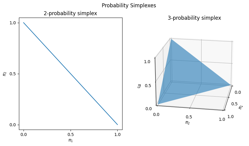
The values of $\overrightarrow{\pi }=(\pi )$ that are in the $K$-probability simplex are indicated by the shaded region of each figure. This comprises the $({\pi }_1,{\pi }_2)$ pairs that fall along a diagonal line from $(0,1)$ to $(1,0)$ for the $2$-simplex, and the $({\pi }_1,{\pi }_2,{\pi }_3)$ tuples that fall on the surface of the triangular shape above with nodes at $(1,0,0)$, $(0,1,0)$, and $(0,0,1)$.

This model has the following parameters:

Parameter	Space	Description
$\overrightarrow{\pi }$	the $K$ probability simplex	The probability of a node being assigned to community $K$
$B$	[0,1]${}^{K\times K}$	The block matrix, which assigns edge probabilities for pairs of communities

The a posteriori SBM is a bit more complicated than the a priori SBM. We will think about the a posteriori SBM as a variation of the a priori SBM, where instead of the node-assignment vector being treated as a known fixed value (the community assignments), we will treat it as unknown. $\overrightarrow{\tau \tau }$ is called a latent variable, which means that it is a quantity that is never actually observed, but which will be useful for describing our model. In this case, $\overrightarrow{\tau \tau }$ takes values in the space $\{1,...,K{\}}^n$. This means that for a given realization of $\overrightarrow{\tau \tau }$, denoted by $\overrightarrow{\tau }$, that for each of the $n$ nodes in the network, we suppose that an integer value between $1$ and $K$ indicates which community a node is from. Statistically, we write that the node assignment for node $i$, denoted by $\tau {\tau }_i$, is sampled independently and identically from $Categorical(\overrightarrow{\pi })$. Stated another way, the vector $\overrightarrow{\pi }$ indicates the probability ${\pi }_k$ of assignment to each community $k$ in the network.

The matrix $B$ behaves exactly the same as it did with the a posteriori SBM. Finally, let’s think about how to write down the generative model in the a posteriori SBM. The model for the a posteriori SBM is, in fact, nearly the same as for the a priori SBM: we still say that given ${\tau }_i=k^{\prime }$ and ${\tau }_j=k$, that ${\mathbf{a}}_{ij}$ are independent $Bern(b_{k^{\prime }k})$. Here, however, we also describe that $\tau {\tau }_i$ are sampled independent and identically from $Categorical(\overrightarrow{\pi })$, as we learned above. If $\mathbf{A}$ is the adjacency matrix for an a posteriori SBM network with parameters $\overrightarrow{\pi }$ and $B$, we write that $\mathbf{A}\sim SB{M}_n(\overrightarrow{\pi },B)$.

11.5.2.1. Probability

What does the probability for the a posteriori SBM look like? In this case, $\theta =(\overrightarrow{\pi },B)$ are the parameters for the model, so the probability for a realization $A$ of $\mathbf{A}$ is:

$$\begin{array}{rl}P{r}_{\theta }(A)& =P{r}_{\theta }(\mathbf{A}=A)\end{array}$$

Next, we use the fact that the probability that $\mathbf{A}=A$ is, in fact, the integration (over realizations of $\overrightarrow{\tau \tau }$) of the joint $(\mathbf{A},\overrightarrow{\tau \tau })$. In this case, we will let $\mathcal{T}=\{1,...,K{\}}^n$ be the space of all possible realizations that $\overrightarrow{\tau \tau }$ could take:

(11.1)$$\begin{array}{rl}P{r}_{\theta }(A)& =\sum _{\overrightarrow{\tau }\in \mathcal{T}}P{r}_{\theta }(\mathbf{A}=A,\overrightarrow{\tau \tau }=\overrightarrow{\tau })\end{array}$$

Next, remember that by definition of a conditional probability for a random variable $\mathbf{x}$ taking value $x$ conditioned on random variable $\mathbf{y}$ taking the value $y$, that $Pr(\mathbf{x}=x|\mathbf{y}=y)=\frac{Pr(\mathbf{x}=x,\mathbf{y}=y)}{Pr(\mathbf{y}=y)}$. Note that by multiplying through by $\mathbf{P}(\mathbf{y}=y)$, we can see that $Pr(\mathbf{x}=x,\mathbf{y}=y)=Pr(\mathbf{x}=x|\mathbf{y}=y)Pr(\mathbf{y}=y)$. Using this logic for $\mathbf{A}$ and $\overrightarrow{\tau \tau }$:

$$\begin{array}{rl}P{r}_{\theta }(A)& =\sum _{\overrightarrow{\tau }\in \mathcal{T}}P{r}_{\theta }(\mathbf{A}=A|\overrightarrow{\tau \tau }=\overrightarrow{\tau })Pr(\overrightarrow{\tau \tau }=\overrightarrow{\tau })\end{array}$$

Intuitively, for each term in the sum, we are treating $\overrightarrow{\tau \tau }$ as taking a fixed value, $\overrightarrow{\tau }$, to evaluate this probability statement.

We will start by describing $Pr(\overrightarrow{\tau \tau }=\overrightarrow{\tau })$. Remember that for $\overrightarrow{\tau \tau }$, that each entry $\tau {\tau }_i$ is sampled independently and identically from $Categorical(\overrightarrow{\pi })$.The probability mass for a $Categorical(\overrightarrow{\pi })$-valued random variable is $Pr(\tau {\tau }_i={\tau }_i;\overrightarrow{\pi })={\pi }_{{\tau }_i}$. Finally, note that if we are taking the products of $n$ ${\pi }_{{\tau }_i}$ terms, that many of these values will end up being the same. Consider, for instance, if the vector $\tau =[1,2,1,2,1]$. We end up with three terms of ${\pi }_1$, and two terms of ${\pi }_2$, and it does not matter which order we multiply them in. Rather, all we need to keep track of are the counts of each $\pi$ term. Written another way, we can use the indicator that ${\tau }_i=k$, given by ${\mathbb{1}}_{{\tau }_i=k}$, and a running counter over all of the community probability assignments ${\pi }_k$ to make this expression a little more sensible. We will use the symbol $n_k=\sum _{i=1}^n{\mathbb{1}}_{{\tau }_i=k}$ to denote this value, which is the number of nodes in community $k$:

$$\begin{array}{rl}P{r}_{\theta }(\overrightarrow{\tau \tau }=\overrightarrow{\tau })& =\prod _{i=1}^{n}P{r}_{\theta }(\tau {\tau }_i={\tau }_i),\text{Independence Assumption}\\ & =\prod _{i=1}^n{\pi }_{{\tau }_i},\text{p.m.f. of a Categorical R.V.}\\ & =\prod _{k=1}^K{\pi }_k^{n_k},\text{Reorganizing what we are taking products of}\end{array}$$

Next, let’s think about the conditional probability term, $P{r}_{\theta }(\mathbf{A}=A|\overrightarrow{\tau \tau }=\overrightarrow{\tau })$. Remember that the entries are all independent conditional on $\overrightarrow{\tau \tau }$ taking the value $\overrightarrow{\tau }$. It turns out this is exactly the same result that we obtained for the a priori SBM:

$$\begin{array}{rl}P{r}_{\theta }(\mathbf{A}=A|\overrightarrow{\tau \tau }=\overrightarrow{\tau })& =\prod _{k^{\prime },k}{b}_{\ell k}^{m_{k^{\prime }k}}(1-b_{k^{\prime }k}{)}^{n_{k^{\prime }k}-m_{k^{\prime }k}}\end{array}$$

Combining these into the integrand gives:

$$\begin{array}{rl}P{r}_{\theta }(A)& =\sum _{\overrightarrow{\tau }\in \mathcal{T}}P{r}_{\theta }(\mathbf{A}=A|\overrightarrow{\tau \tau }=\overrightarrow{\tau })P{r}_{\theta }(\overrightarrow{\tau \tau }=\overrightarrow{\tau })\\ & =\sum _{\overrightarrow{\tau }\in \mathcal{T}}\prod _{k=1}^K[{\pi }_k^{n_k}\cdot \prod _{k^{\prime }=1}^K{b}_{k^{\prime }k}^{m_{k^{\prime }k}}(1-b_{k^{\prime }k}{)}^{n_{k^{\prime }k}-m_{k^{\prime }k}}]\end{array}$$

Evaluating this sum explicitly proves to be relatively tedious and is a bit outside of the scope of this book, so we will omit it here.

11.5.3. Degree-Corrected Stochastic Block Model (DCSBM)

Let’s think back to our school example for the Stochastic Block Model. Remember, we had 100 students, each of whom could go to one of two possible schools: school one or school two. Our network had 100 nodes, representing each of the students. We said that the school for which each student attended was represented by their node assignment ${\tau }_i$ to one of two possible communities. The matrix $B$ was the block probaability matrix, where $b_{11}$ was the probability that students in school one were friends, $b_{22}$ was the probability that students in school two were friends, and $b_{12}=b_{21}$ was the probability that students were friends if they did not go to the same school. In this case, we said that $\mathbf{A}$ was an $SB{M}_n(\tau ,B)$ random network.

When would this setup not make sense? Let’s say that Alice and Bob both go to the same school, but Alice is more popular than Bob. In general since Alice is more popular than Bob, we might want to say that for any clasasmate, Alice gets an additional “popularity benefit” to her probability of being friends with the other classmate, and Bob gets an “unpopularity penalty.” The problem here is that within a single community of an SBM, the SBM assumes that the node degree (the number of nodes each nodes is connected to) is the same for all nodes within a single community. This means that we would be unable to reflect this benefit/penalty system to Alice and Bob, since each student will have the same number of friends, on average. This problem is referred to as community degree homogeneity in a Stochastic Block Model Network. Community degree homogeneity just means that the node degree is homogeneous, or the same, for all nodes within a community.

Degree Homogeneity in a Stochastic Block Model Network

Suppose that $\mathbf{A}\sim SB{M}_{n,\overrightarrow{\tau }}(B)$, where $\mathbf{A}$ has $K=2$ communities. What is the node degree of each node in $\mathbf{A}$?

For an arbitrary node $v_i$ which is in community $k$ (either one or two), we will compute the expectated value of the degree $deg(v_i)$, written $\mathbb{E}[deg(v_i);{\tau }_i=k]$. We will let $n_k$ represent the number of nodes whose node assignments ${\tau }_i$ are to community $k$. Let’s see what happens:

$$\begin{array}{rl}\mathbb{E}[deg(v_i);{\tau }_i=k]& =\mathbb{E}\left[\sum _{j=1}^n{\mathbf{a}}_{ij}\right]\\ & =\sum _{j=1}^n\mathbb{E}[{\mathbf{a}}_{ij}]\end{array}$$

We use the linearity of expectation again to get from the top line to the second line. Next, instead of summing over all the nodes, we’ll break the sum up into the nodes which are in the same community as node $i$, and the ones in the other community $k^{\prime }$. We use the notation $k^{\prime }$ to emphasize that $k$ and $k^{\prime }$ are different values:

$$\begin{array}{rl}\mathbb{E}[deg(v_i);{\tau }_i=k]& =\sum _{j:i\ne j,{\tau }_j=k}\mathbb{E}\left[{\mathbf{a}}_{ij}\right]+\sum _{j:{\tau }_j=k^{\prime }}\mathbb{E}[{\mathbf{a}}_{ij}]\end{array}$$

In the first sum, we have $n_k-1$ total edges (the number of nodes that aren’t node $i$, but are in the same community), and in the second sum, we have $n_{k^{\prime }}$ total edges (the number of nodes that are in the other community). Finally, we will use that the probability of an edge in the same community is $b_{kk}$, but the probability of an edge between the communities is $b_{k^{\prime }k}$. Finally, we will use that the expected value of an adjacency ${\mathbf{a}}_{ij}$ which is Bernoulli distributed is its probability:

$$\begin{array}{rl}\mathbb{E}[deg(v_i);{\tau }_i=k]& =\sum _{j:i\ne j,{\tau }_j=k}{b}_{kk}+\sum _{j:{\tau }_j=\ell }{b}_{k{k}^{\prime }},{\mathbf{a}}_{ij}\text{ are Bernoulli distributed}\\ & =(n_k-1)b_{kk}+n_{k^{\prime }}{b}_{k{k}^{\prime }}\end{array}$$

This holds for any node $i$ which is in community $k$. Therefore, the expected node degree is the same, or homogeneous, within a community of an SBM.

To address this limitation, we turn to the Degree-Corrected Stochastic Block Model, or DCSBM. As with the Stochastic Block Model, there is both a a priori and a posteriori DCSBM.

11.5.3.1. A Priori DCSBM

Like the a priori SBM, the a priori DCSBM is where we know which nodes are in which communities ahead of time. Here, we will use the variable $K$ to denote the number of different communiies. The a priori DCSBM has the following two parameters:

Parameter	Space	Description
$B$	[0,1]${}^{K\times K}$	The block matrix, which assigns edge probabilities for pairs of communities
$\overrightarrow{\theta }$	${\mathbb{R}}_{+}^n$	The degree correction vector, which adjusts the degree for pairs of nodes

The latent community assignment vector $\overrightarrow{\tau \tau }$ with a known a priori realization $\overrightarrow{\tau }$ and the block matrix $B$ are exactly the same for the a priori DCSBM as they were for the a priori SBM.

The vector $\overrightarrow{\theta }$ is the degree correction vector. Each entry ${\theta }_i$ is a positive scalar. ${\theta }_i$ defines how much more (or less) edges associated with node $i$ are connected due to their association with node $i$.

Finally, let’s think about how to write down the generative model for the a priori DCSBM. We say that ${\tau }_i=k^{\prime }$ and ${\tau }_j=k$, ${\mathbf{a}}_{ij}$ is sampled independently from a $Bern({\theta }_i{\theta }_j{b}_{k^{\prime }k})$ distribution for all $j>i$. As we can see, ${\theta }_i$ in a sense is “correcting” the probabilities of each adjacency to node $i$ to be higher, or lower, depending on the value of ${\theta }_i$ that that which is given by the block probabilities $b_{\ell k}$. If $\mathbf{A}$ is an a priori DCSBM network with parameters and $B$, we write that $\mathbf{A}\sim DCSB{M}_{n,\overrightarrow{\tau }}(\overrightarrow{\theta },B)$.

11.5.3.1.1. Probability

The derivation for the probability is the same as for the a priori SBM, with the change that $p_{ij}={\theta }_i{\theta }_j{b}_{k^{\prime }k}$ instead of just $b_{k^{\prime }k}$. This gives that the probability turns out to be:

$$\begin{array}{rl}P{r}_{\theta }(A)& =\prod _{j>i}{\left({\theta }_i{\theta }_j{b}_{k^{\prime }k}\right)}^{a_{ij}}{(1-{\theta }_i{\theta }_j{b}_{k^{\prime }k})}^{1-a_{ij}}\end{array}$$

The expression doesn’t simplify much more due to the fact that the probabilities are dependent on the particular $i$ and $j$, so we can’t just reduce the statement in terms of $n_{k^{\prime }k}$ and $m_{k^{\prime }k}$ like for the SBM.

11.5.3.2. A Posteriori DCSBM

The a posteriori DCSBM is to the a posteriori SBM what the a priori DCSBM was to the a priori SBM. The changes are very minimal, so we will omit explicitly writing it all down here so we can get this section wrapped up, with the idea that the preceding section on the a priori DCSBM should tell you what needs to change. We will leave it as an exercise to the reader to write down a model and probability statement for realizations of the DCSBM.