Discover and Visualize the Data to Gain Insights
Contents
2.6. Discover and Visualize the Data to Gain Insights#
So, now we’ve got a codebase accumulated to read in the input data, get it cleaned up, embed it while borrowing strength from all networks, and make some predictions:
import warnings
warnings.filterwarnings("ignore")
import os
import urllib
import boto3
from botocore import UNSIGNED
from botocore.client import Config
from graspologic.utils import import_edgelist, pass_to_ranks
import numpy as np
from sklearn.base import TransformerMixin, BaseEstimator
from sklearn.pipeline import Pipeline
import glob

# the AWS bucket the data is stored in
BUCKET_ROOT = "open-neurodata"
# the path to the data we are interested in
parcellation = "Schaefer400"
FMRI_PREFIX = "m2g/Functional/BNU1-11-12-20-m2g-func/Connectomes/" + \
    parcellation + "_space-MNI152NLin6_res-2x2x2.nii.gz/"
FMRI_PATH = os.path.join("datasets", "fmri")  # the output folder
DS_KEY = "abs_edgelist"  # correlation matrices for the networks to exclude

def fetch_fmri_data(bucket=BUCKET_ROOT, fmri_prefix=FMRI_PREFIX,
                    output=FMRI_PATH, name=DS_KEY):
    """
    A function to fetch fMRI connectomes from AWS S3.
    """
    # check that output directory exists
    if not os.path.isdir(FMRI_PATH):
        os.makedirs(FMRI_PATH)
    # start boto3 session anonymously
    s3 = boto3.client('s3', config=Config(signature_version=UNSIGNED))
    # obtain the filenames
    bucket_conts = s3.list_objects(Bucket=bucket,
                    Prefix=fmri_prefix)["Contents"]
    for s3_key in bucket_conts:
        # get the filename
        s3_object = s3_key['Key']
        # verify that we are grabbing the right file
        if name not in s3_object:
            op_fname = os.path.join(FMRI_PATH, str(s3_object.split('/')[-1]))
            if not os.path.exists(op_fname):
                s3.download_file(bucket, s3_object, op_fname)

def read_fmri_data(path=FMRI_PATH):
    """
    A function which loads the connectomes as adjacency matrices.
    """
    # import edgelists with graspologic
    # edgelists will be all of the files that end in a csv
    networks = [import_edgelist(fname) for fname in glob.glob(os.path.join(path, "*.csv"))]
    return networks

def remove_isolates(A):
    """
    A function which removes isolated nodes from the
    adjacency matrix A.
    """
    degree = A.sum(axis=0)  # sum along the rows to obtain the node degree
    out_degree = A.sum(axis=1)
    A_purged = A[~(degree == 0),:]
    A_purged = A_purged[:,~(degree == 0)]
    print("Purging {:d} nodes...".format((degree == 0).sum()))
    return A_purged

class CleanData(BaseEstimator, TransformerMixin):
    def __init__(self):
        return
    def fit(self, X):
        return self

    def transform(self, X):
        print("Cleaning data...")
        Acleaned = remove_isolates(X)
        A_abs_cl = np.abs(Acleaned)
        self.A_ = A_abs_cl
        return self.A_

class FeatureScaler(BaseEstimator, TransformerMixin):
    def __init__(self):
        return

    def fit(self, X):
        return self

    def transform(self, X):
        print("Scaling edge-weights...")
        A_scaled = pass_to_ranks(X)
        return (A_scaled)

num_pipeline = Pipeline([
    ('cleaner', CleanData()),
    ('scaler', FeatureScaler()),
])
import contextlib

fetch_fmri_data()

As_raw = read_fmri_data()
with contextlib.redirect_stdout(None):
    As = np.stack([num_pipeline.fit_transform(A) for A in As_raw], axis=0)
from graspologic.embed import MultipleASE
from graspologic.cluster import AutoGMMCluster

embedding = MultipleASE().fit_transform(As)
labels = AutoGMMCluster(max_components=10).fit_predict(embedding)
So, now you’re finished, right?
Wrong! The end of a computational analysis typically means the fun is just beginning: it’s now time to make sense of whatever, exactly, it is that you just did!
How could we visualize the node clusters (or, more formally, called communities) that we just made? We already know about the pairplot:
from graspologic.plot import pairplot

_ = pairplot(embedding, labels=labels, legend_name="Predicted Community", title="MASE of connectomes")
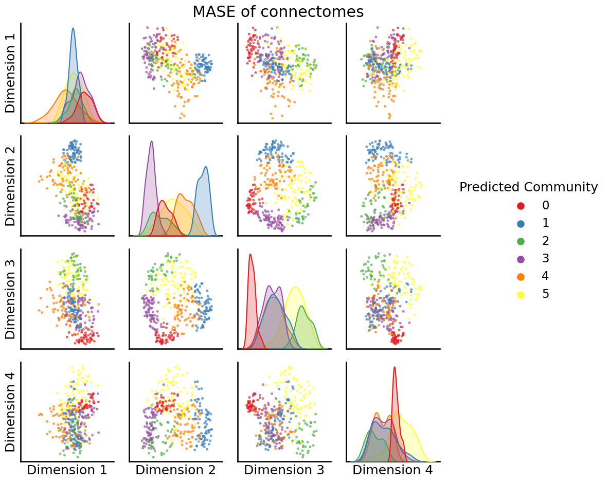
What if we take a look at the nodes, which if we remember were areas of the brain, how they really look in the brain’s natural space?
It turns out that the areas of the brain for your network are, in fact, known 3D points in the brain. This means that, with some minor work, we can figure out the coordinates of the individual nodes for the brain. Let’s use the neuroparc repository from [1] to grab the 3D coordinates of each node in the network:
from urllib import request
import json
import pandas as pd

coord_dest = os.path.join(FMRI_PATH, "coordinates.json")
request.urlretrieve("https://github.com/neurodata/neuroparc/raw/master/atlases/label/Human/Metadata-json/" +
                    parcellation + "_space-MNI152NLin6_res-2x2x2.json",
                    coord_dest);
coord_f = open(coord_dest)

coords = []
for roiname, contents in json.load(coord_f)["rois"].items():
    try:
        if roiname != "0":
            coord_roi = {"x" : contents["center"][0], "y" : contents["center"][1], "z" : contents["center"][2]}
            coords.append(coord_roi)
    except:
        continue
coords_df = pd.DataFrame(coords)
Now that we have the coordinates, let’s try plotting the nodes, but in their native spatial orientation. Here, the color will indicate the predicted label, from our clustering. The slices we’ll show will be a saggital slice through the brain. A saggital slice shows the brain nodes oriented from back (right of the plot) of the brain to front (left of the plot), and from bottom (bottom of the plot) to top (top of the plot). On the left, we show the brain with the lobe annotations, and on the right, the predicted labels of each node in color, where each node is shown in its true physical location:
import matplotlib.pyplot as plt
import seaborn as sns
import matplotlib.image as mpimg

coords_df["Community"] = labels
coords_df['Community'] = coords_df['Community'].astype('category')
fig, axs = plt.subplots(1, 2, figsize=(18, 6))
axs[0].imshow(mpimg.imread('./Images/lobes.png'))
axs[0].set_axis_off()
sns.scatterplot(x="y", y="z", data=coords_df, hue="Community", ax=axs[1])
fig;
So, the colors of the brain areas don’t quite perfectly align with the brain lobe, although as we can see above, nodes in the same community are often near nodes within that same community (notice, for instance, that a lot of nodes in the left side of the brain, the part marked “occipital lobe” in the plot, tend to be the same color).
In neuroimaging, there tend to be “groups” of brain areas that work together, which are organized in files called “parcellations”. The idea is that they “parcellate” (segment) different areas of the brain baesd on two factors: whether the areas of the brain work together, and whether they are located near each other in the brain. Let’s see how well the labels we obtained align with these parcellations. We’ll do this by looking at the different parcellations (there are \(7\) of them in the one that we will use here), and count the number of nodes in a given community (the thing that you just estimated, indicated by color, above) that are assigned to a particular parcel as well. This means that we will end up with a matrix where the number of rows are the number of true parcels in the brain, the number of columns is the number of predicted communities that you found above, and the entries of the matrix are the counts of nodes in the network that are assigned to a given community and fall into a given parcel:
import contextlib
import datasets.dice as dice
from sklearn.metrics import confusion_matrix
from graphbook_code import cmaps

group_dest = os.path.join("./datasets/", "Yeo-7_space-MNI152NLin6_res-2x2x2.nii.gz")
request.urlretrieve("https://github.com/neurodata/neuroparc/blob/master/atlases/label/Human/" +
                    "Yeo-7_space-MNI152NLin6_res-2x2x2.nii.gz?raw=true",
                    group_dest);
roi_dest = os.path.join("./datasets/", "Schaefer200_space-MNI152NLin6_res-2x2x2.nii.gz")
request.urlretrieve("https://github.com/neurodata/neuroparc/blob/master/atlases/label/Human/" +
                    "Schaefer400_space-MNI152NLin6_res-2x2x2.nii.gz?raw=true",
                    roi_dest);

dicemap, _, _ = dice.dice_roi("./datasets/", "./datasets", "Yeo-7_space-MNI152NLin6_res-2x2x2.nii.gz",
              "Schaefer200_space-MNI152NLin6_res-2x2x2.nii.gz", verbose=False, plot=False)
actual_cluster = np.argmax(dicemap, axis=0)[1:] - 1

# make confusion matrix
cf_matrix = confusion_matrix(actual_cluster, labels)
---------------------------------------------------------------------------
ExpiredDeprecationError                   Traceback (most recent call last)
Cell In[8], line 15
     10 roi_dest = os.path.join("./datasets/", "Schaefer200_space-MNI152NLin6_res-2x2x2.nii.gz")
     11 request.urlretrieve("https://github.com/neurodata/neuroparc/blob/master/atlases/label/Human/" +
     12                     "Schaefer400_space-MNI152NLin6_res-2x2x2.nii.gz?raw=true",
     13                     roi_dest);
---> 15 dicemap, _, _ = dice.dice_roi("./datasets/", "./datasets", "Yeo-7_space-MNI152NLin6_res-2x2x2.nii.gz",
     16               "Schaefer200_space-MNI152NLin6_res-2x2x2.nii.gz", verbose=False, plot=False)
     17 actual_cluster = np.argmax(dicemap, axis=0)[1:] - 1
     19 # make confusion matrix

File ~/work/graph-stats-book/graph-stats-book/network_machine_learning_in_python/foundations/ch2/datasets/dice.py:32, in dice_roi(input_dir, output_dir, atlas1, atlas2, verbose, plot)
     29 at1 = nb.load(f'{input_dir}/{atlas1}')
     30 at2 = nb.load(f'{input_dir}/{atlas2}')
---> 32 atlas1 = at1.get_data()
     33 atlas2 = at2.get_data()
     35 labs1 = np.unique(atlas1)

File /opt/hostedtoolcache/Python/3.8.16/x64/lib/python3.8/site-packages/nibabel/deprecator.py:185, in Deprecator.__call__.<locals>.deprecator.<locals>.deprecated_func(*args, **kwargs)
    182 @functools.wraps(func)
    183 def deprecated_func(*args, **kwargs):
    184     if until and self.is_bad_version(until):
--> 185         raise error_class(message)
    186     warnings.warn(message, warn_class, stacklevel=2)
    187     return func(*args, **kwargs)

ExpiredDeprecationError: get_data() is deprecated in favor of get_fdata(), which has a more predictable return type. To obtain get_data() behavior going forward, use numpy.asanyarray(img.dataobj).

* deprecated from version: 3.0
* Raises <class 'nibabel.deprecator.ExpiredDeprecationError'> as of version: 5.0
fig, ax = plt.subplots(1,1, figsize=(6,4))
sns.heatmap(cf_matrix, cmap=cmaps["sequential"], ax=ax)
ax.set_title("Confusion matrix")
ax.set_ylabel("True Label")
ax.set_xlabel("Predicted Label")
fig
As you will learn in the section on mase embedding in Section 5.4.4, the mase embedding followed by clustering tends to find groups of nodes that have similar connectivity patterns in the connectomes (it will do a good job at finding the nodes that work together). This means that the nodes in the same community tend to behave “as a unit”, if you will, in that they tend to be active/inactive together. Basically, what the plot above shows is that nodes that tend to have similar connectivity patterns (from the networks) tend to also be in the same parcel (the true label), which makes sense since the parcels are based on connectivity profiles from brains. The clustering isn’t perfect, in that it is never the case that a single predicted label corresponds to exactly one true label. If that were the case, we would expect for each column in the above “confusion matrix” to only have one possible true label that nodes within this predicted label are assigned to, which isn’t quite the case.
Taking these conclusions together, we find that some areas of the brain (such as the occipital and parietal areas) feature nodes which are both functionally and spatially similar: they tend to show similar connectivity patterns with respect to other groups of nodes in the network, and are in similar spatial positions in the brain. On the other hand, for other areas of the brain, while the nodes may be functionally similar, they might not necessarily be spatially similar. This is where the domain expertise kicks in: we don’t know how to interpret this particular aspect of our finding, but maybe you or your colleagues do!
Further, while this analysis only really ended up looking at whether different groups of nodes worked together, there’s really no reason we couldn’t also incorporate spatial information about the nodes into our analysis. In Section 5.5, you will learn some techniques for incorporating both the network data itself and other information about the nodes into your analysis through a technique called Covariate-Assisted Spectral Embedding (CASE).
And this is where the fun of network machine learning comes into play: it is a tool not only to apply algorithms to data, but to facilitate learning new things about that data as well. You might get some predictable conclusions (such as some of the nodes being both functionally and spatially similar), and you might get some unpredictable conclusions (such as some of the nodes being functionally, but not spatially, similar). Your ability to understand network machine learning, while crucial, is going to go hand in hand with your ability to understand the intricacies of the domain you want to apply network machine learning to. We hope that we can help with the former part; we’ll leave the latter to you!
2.6.1. Try it out!#
Hopefully this chapter gave you a small scale peek at what a network machine learning project looks like, and showed you a brief introduction to some tools you can use to gain novel insights from your network data. While what we did in this chapter was relatively straightforward, the process from obtaining your data to choosing appropriate network machine learning problems can be extremely arduous! In fact, as a network machine learning scientist, you might find that just obtaining your data in a useful form (a network) and cleaning the data to be usable might take an enormous chunk of your time!
If you haven’t already done so, now is a fantastic time to grab your laptop, select a network dataset you are interested in, and start trying to work through the whole process from A to Z. If you need some pointers, the graspologic package makes several datasets available to you [2]. We’d recommend working through the contents of this book by first using the example data that is presented in the chapter, and then try to apply the techniques to a network dataset of your choosing.
2.6.2. References#
- 1
Ross M. Lawrence, Eric W. Bridgeford, Patrick E. Myers, Ganesh C. Arvapalli, Sandhya C. Ramachandran, Derek A. Pisner, Paige F. Frank, Allison D. Lemmer, Aki Nikolaidis, and Joshua T. Vogelstein. Standardizing human brain parcellations. Sci. Data, 8(78):1–9, March 2021. doi:10.1038/s41597-021-00849-3.
- 2
Microsoft. Datasets - graspologic 2.0.1 documentation. January 2023. [Online; accessed 4. Feb. 2023]. URL: https://microsoft.github.io/graspologic/latest/reference/reference/datasets.html.