4.4. Inhomogeneous Erdos Renyi (IER) Random Network Model

Now that you’ve learned about the ER, SBM, and RDPG random networks, it’s time to figure out why we keep using coin flips! To this end, you will learn about the most general model for an independent edge random network, the Inhomogeneous Erdos Renyi (IER) Random Network.

Click to show

import numpy as np
from graspologic.simulations import sample_edges
from graphbook_code import draw_multiplot

def my_unit_circle(r):
   d = 2*r + 1
   rx, ry = d/2, d/2
   x, y = np.indices((d, d))
   return (np.abs(np.hypot(rx - x, ry - y)-r) < 0.5).astype(int)

def add_smile():
    Ptmp = np.zeros((51, 51))
    Ptmp[2:45, 2:45] = my_unit_circle(21)
    mask = np.zeros((51, 51), dtype=bool)
    mask[np.triu_indices_from(mask)] = True
    upper_left = np.rot90(mask)
    Ptmp[upper_left] = 0
    return Ptmp
    
def smiley_prob(upper_p, lower_p):
    smiley = add_smile()
    P = my_unit_circle(25)
    P[5:16, 25:36] = my_unit_circle(5)
    P[smiley != 0] = smiley[smiley != 0]
    
    mask = np.zeros((51, 51), dtype=bool)
    mask[np.triu_indices_from(mask)] = True
    P[~mask] = 0
    P = (P + P.T - np.diag(np.diag(P))).astype(float)
    P[P == 1] = lower_p
    P[P == 0] = upper_p
    return P

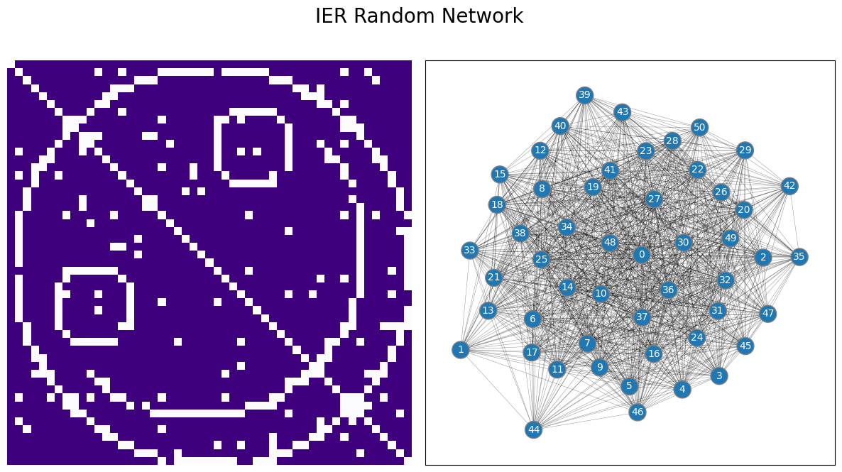
P = smiley_prob(.95, 0.05)
A = sample_edges(P, directed=False, loops=False)

draw_multiplot(A, title="IER Random Network");

4.4.1. The Inhomogeneous Erdos-Renyi (IER) Random Network Model is parametrized by a matrix of independent-edge probabilities

The IER random network is the most general random network model for a binary graph. The way you can think of the IER random network is that a probability matrix $P$ with $n$ rows and $n$ columns defines each of the edge-existence probabilities for pairs of nodes in the network. For each pair of nodes $i$ and $j$, you have a unique coin which has a $p_{ij}$ chance of landing on heads, and a $1-p_{ij}$ chance of landing on tails. If the coin lands on heads, the edge between nodes $i$ and $j$ exists, and if the coin lands on tails, the edge between nodes $i$ and $j$ does not exist. This coin flip is performed independently of the coin flips for all of the other edges. If $\mathbf{A}$ is a random network which is $IER$ with a probability matrix $P$, we say that $\mathbf{A}$ is an $IE{R}_n(P)$ random network.

4.4.1.1. Generating a sample from an $IE{R}_n(P)$ random network

As before, you can develop a procedure to produce for you a network $A$, which has nodes and edges, where the underlying random network $\mathbf{A}$ is an $IE{R}_n(P)$ random network:

Simulating a sample from an $IE{R}_n(P)$ random network

1. Choose a probability matrix $P$, whose entries $p_{ij}$ are probabilities.

2. For each pair of nodes $i$ an $j$:

   • Obtain a weighted coin $(i,j)$ which has a probability $p_{ij}$ of landing on heads, and a $1-p_{ij}$ probability of landing on tails.

   • Flip the $(i,j)$ coin, and if it lands on heads, the corresponding entry $a_{ij}$ in the adjacency matrix is $1$. If the coin lands on tails, the corresponding entry $a_{ij}$ is $0$.

3. The adjacency matrix you produce, $A$, is a sample of an $IE{R}_n(P)$ random network.

Let’s put this in practice. Since you know about probability matrices from the section on RDPG, you’ll first take a look at the probability matrix for your IER network. This example is very unnecessarily sophisticated, but we have a reason for it:

import numpy as np

def my_unit_circle(r):
   d = 2*r + 1
   rx, ry = d/2, d/2
   x, y = np.indices((d, d))
   return (np.abs(np.hypot(rx - x, ry - y)-r) < 0.5).astype(int)

def add_smile():
    Ptmp = np.zeros((51, 51))
    Ptmp[2:45, 2:45] = my_unit_circle(21)
    mask = np.zeros((51, 51), dtype=bool)
    mask[np.triu_indices_from(mask)] = True
    upper_left = np.rot90(mask)
    Ptmp[upper_left] = 0
    return Ptmp
    
def smiley_prob(upper_p, lower_p):
    smiley = add_smile()
    P = my_unit_circle(25)
    P[5:16, 25:36] = my_unit_circle(5)
    P[smiley != 0] = smiley[smiley != 0]
    
    mask = np.zeros((51, 51), dtype=bool)
    mask[np.triu_indices_from(mask)] = True
    P[~mask] = 0
    P = (P + P.T - np.diag(np.diag(P))).astype(float)
    P[P == 1] = lower_p
    P[P == 0] = upper_p
    return P

P = smiley_prob(.95, 0.05)

Click to show

from graphbook_code import heatmap

ax = heatmap(P, vmin=0, vmax=1, title="Probability matrix for smiley face example")
ax.set_xlabel("Node")
ax.set_ylabel("Node");

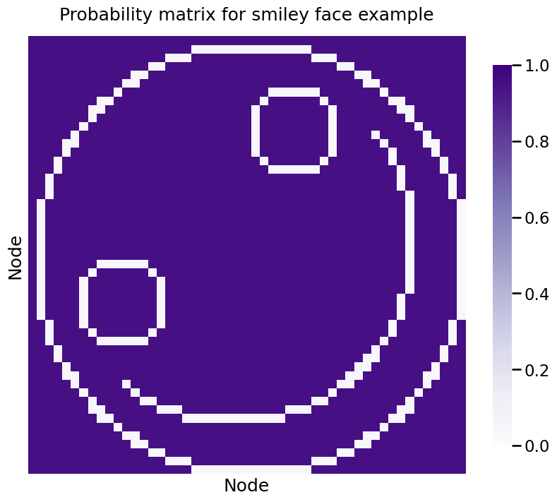
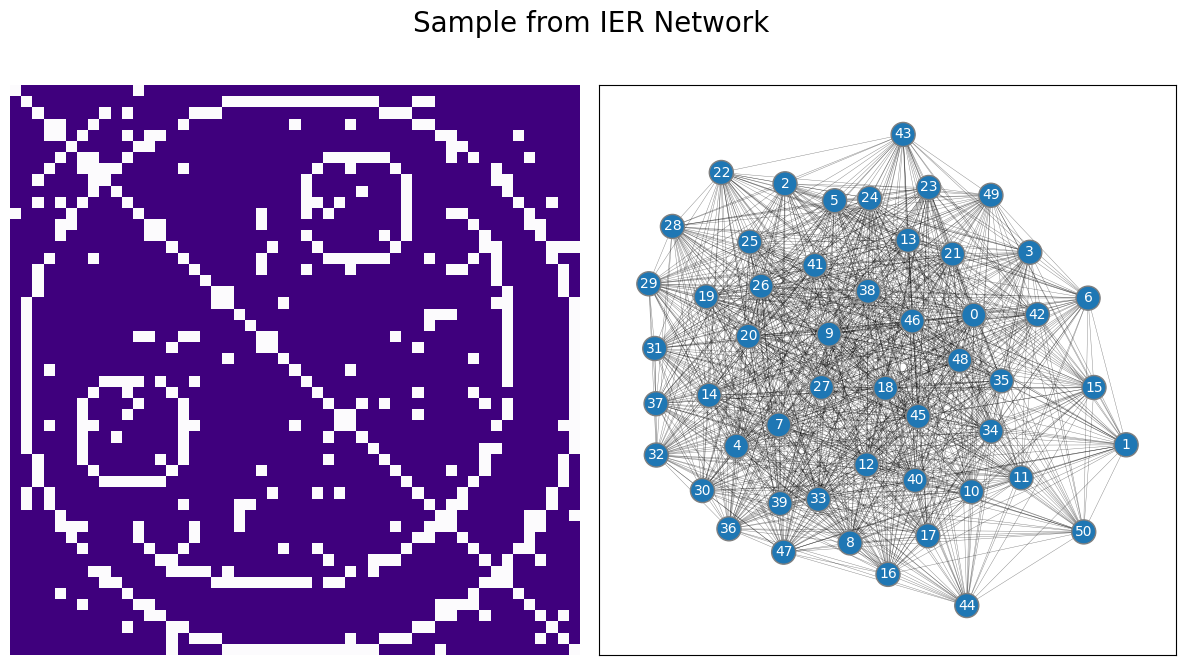
If the edge is between a pair of nodes that defines the smiley face, the probability is $0.05$, whereas the edge probability for the other edges in the network is $0.95$. A network realization looks like this:

A = sample_edges(P, directed=False, loops=False)

Click to show

draw_multiplot(A, title="Sample from IER Network");

We used this example to show you the key idea behind the IER Network’s probability matrix is simple: the entries can really be anything as long as they are probabilities (between $0$ and $1$), and the resulting matrix is symmetric (in the case of undirected networks). There are no additional requirements for structure to the network.

4.4.2. The IER model unifies independent-edge random network models

It is important to realize that all of the networks you have learned so far are also IER random networks. The previous single network models you have covered to date simply place restrictions on the way in which you acquire $P$. For instance, in an $E{R}_n(p)$ random network, all entries $p_{ij}$ of $P$ can just be set equal to $p$. To see that an $SB{M}_n(\overrightarrow{z},B)$ random network is also $IE{R}_n(P)$, you can construct the probability matrix $P$ such that $p_{ij}=b_{kl}$ of the block matrix $B$ when the community of node $i$ is $z_i=k$ and the community of node $j$ is $z_j=l$. To see that an $RDP{G}_n(X)$ random network is also $IE{R}_n(P)$, you can construct the probability matrix $P$ such that $P=X{X}^{\mathrm{\top }}$. This shows that the IER random network is the most general of the single network models you have studied so far.

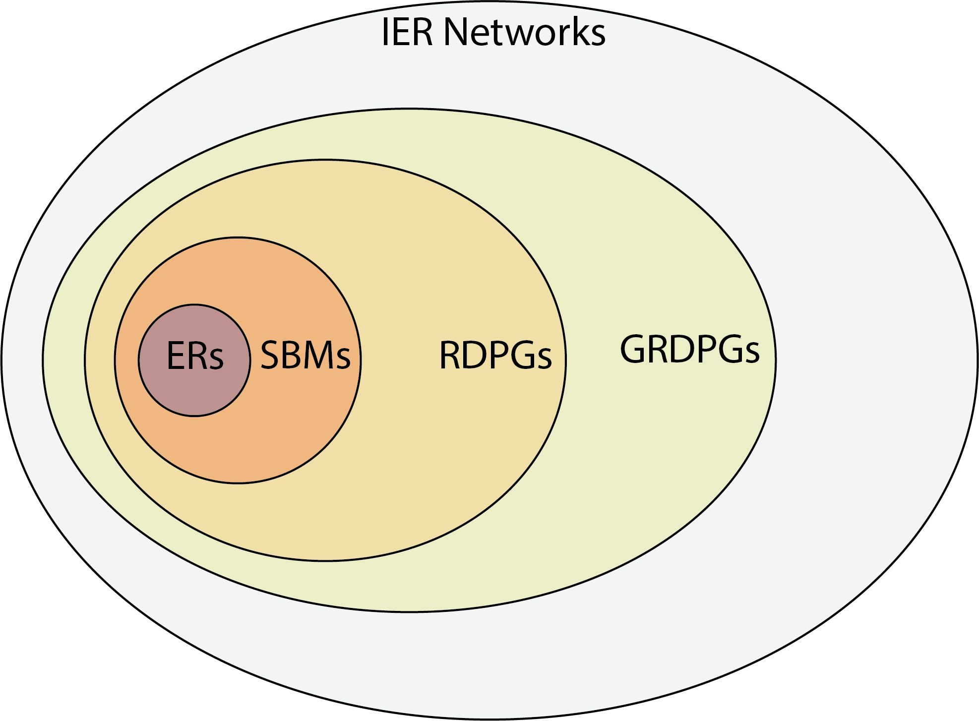
Fig. 4.2 The IER network unifies independent-edge random networks, as it is the most general independent-edge random network model. What this means is that all models discussed so far, and many not discussed but found in the appendix, can be conceptualized as special cases of the IER network. Stated in other words, a probability matrix is the fundamental unit necessary to describe an independent-edge random network model. For the models covered so far, all GRDPGs are IER networks (by taking $P$ to be $X{Y}^{\mathrm{\top }}$), all RDPGs are GRDPGs (by taking the right latent positions $Y$ to be equal to the left latent positions $X$), all SBMs are RDPGs, and all ERs are SBMs, whereas the converses in general are not true.

4.4.2.1. How do you obtain a probability matrix for an SBM programmatically?

One thing that will come up frequently over the course of this book is that we will need to sometimes programmatically generate the probability matrix directly (rather than just using the community assignment vector $\overrightarrow{z}$ and the block probability matrix $B$). This isn’t too difficult to do.

Basically, the idea is as follows. If $\overrightarrow{z}$ is the community assignment vector and assigns the $n$ nodes of the network to one of $K$ communities (taking values from $1$, $2$, …, $K$), and $B$ is the $K\times K$ block probability matrix:

1. You begin by constructing a matrix, $Z$, that has $n$ rows and $K$ columns; one row for each node, and one column for each community.

2. For each node in the network $i$:

   • For each community in the network $k$, if $z_i=k$, then let $z_{ik}=1$. if $z_i\ne k$, then let $z_{ik}=0$.

3. Let $P=ZB{Z}^{\mathrm{\top }}$.

The matrix produced, $P$, is the full probability matrix for the SBM, where entry $p_{ij}$ is the probability that node $i$ is connected to node $j$.

Let’s work through this example programmatically, because it comes up a few times over the course of the book. Let’s imagine that we have $50$ nodes, of which the first $25$ are in community one and the second $25$ are in community two. The code to do this conversion looks like this:

def make_community_mtx(z):
    """
    A function to generate the one-hot-encoded community
    assignment matrix from a community assignment vector.
    """
    K = len(np.unique(z))
    n = len(z)
    Z = np.zeros((n, K))
    for i, zi in enumerate(z):
        Z[i, zi - 1] = 1
    return Z

# the community assignment vector
z = [1 for i in range(0, 25)] + [2 for i in range(0, 25)]
Z = make_community_mtx(z)
# block matrix
B = np.array([[0.6, 0.3], [0.3, 0.6]])
# probability matrix
P = Z @ B @ Z.T

4.4.2.2. Limitations of the IER model when you have one network

This construction is not entirely useful when you have one sample, because for each edge, you only get to see one sample (either the edge exists or doesn’t exist). This means that you won’t really be able to learn about the individual edge probabilities in practice when you only have a single sample of a network in a way which would differentiate them from other single networks. What we mean by this is, if you learn about other single networks, you are still technically learning about an IER random network, because like you saw in the last paragraph, all of these other single network models are just special cases of the IER random network. However, you can’t learn any random network with one sample that could only be described by an IER random network, so it almost feels a little bit useless from what you’ve covered so far. As you will learn shortly, the IER random network is, on the other hand, extremely useful when you have multiple networks. When you have multiple networks, with some limited assumptions, you can learn about networks that you would otherwise not be able to describe with more simple random networks like ER, SBM, or RDPG random netweorks. This will make the IER random network extremely powerful when you have multiple samples of network data.

4.4.3. References

The survey paper [3] and the appendix section Section 11.3 give an overview of the theoretical properties of IER networks.

1

Avanti Athreya, Donniell E. Fishkind, Minh Tang, Carey E. Priebe, Youngser Park, Joshua T. Vogelstein, Keith Levin, Vince Lyzinski, and Yichen Qin. Statistical inference on random dot product graphs: a survey. J. Mach. Learn. Res., 18(1):8393–8484, January 2017. doi:10.5555/3122009.3242083.