7.2. Two-sample hypothesis testing in SBMs

In the previous section, we saw a situation where we had two networks which we thought could be effectively characterized with RDPG. Further, we knew that the communities were the same across both networks: that is, we knew that community \(1\) in the first network was the same as community \(1\) in the second network, so on and so forth all the way up to community \(K\). In this situation, we found that we could test whether the latent positions for the underlying RDPGs are the same; that is, whether \(H_0: X_1 = X_2R\) against \(H_A: H_1 \neq X_2R\). We called this the two-sample hypothesis test for RDPGs.

What if we can take this a step further, however, and we can say that the networks are realizations of SBMs? How can we check whether the block matrices are the same? If you remember from Section 4.3, we learned that SBMs are also RDPGs. What this means is that, since the SBM is an RDPG, the SBM also has a latent position matrix. Therefore, we could test whether the networks are the same by just using the two-sample hypothesis test for the RDPG in Section 7.1. The interpretation of rejecting, or failing to reject, the null hypothesis here was that the latent positions were the same/different across the two networks, and therefore, they share the same probability matrix. This is excellent news, so are we done?

Not quite yet; as it turns out, when we think that the networks are realizations of SBMs, there are a lot more interesting questions we can ask about the probabilities that might arise. Specifically, we can deduce many useful ways in which two probability matrices for SBMs might be different, but still share similar characteristics.

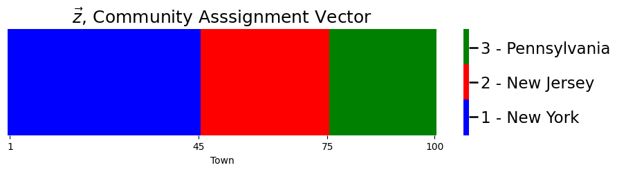
For this example, we will introduce a new scenario. We have two networks which summarize the traffic patterns between \(n=100\) towns (represented by the nodes in our network) across \(K=3\) states (represented by the communities in our network). The first 45 towns are in New York (the first community), the second 30 towns are in New Jersey (the second community), and the third 25 towns are in Pennsylvania (the third community). The community assignment vector \(\vec z\) looks like this:

import numpy as np

ns = [45, 30, 25]  # number of students

# z is a column vector indicating which state each
# town is in
z = np.array([1 for i in range(0, ns[0])] + 
              [2 for i in range(0, ns[1])] +
              [3 for i in range(0, ns[2])] )

import matplotlib.pyplot as plt
import seaborn as sns
import matplotlib

def plot_tau(tau, title="", xlab="Node"):
    cmap = matplotlib.colors.ListedColormap(["blue", 'red', 'green'])
    fig, ax = plt.subplots(figsize=(10,2))
    with sns.plotting_context("talk", font_scale=1):
        ax = sns.heatmap((tau - 1).reshape((1,tau.shape[0])), cmap=cmap,
                        ax=ax, cbar_kws=dict(shrink=1), yticklabels=False,
                        xticklabels=False)
        ax.set_title(title)
        cbar = ax.collections[0].colorbar
        cbar.set_ticks([.35, 1, 1.65])
        cbar.set_ticklabels(['1 - New York', '2 - New Jersey', '3 - Pennsylvania'])
        ax.set(xlabel=xlab)
        ax.set_xticks([.5,44.5, 74.5,99.5])
        ax.set_xticklabels(["1", "45", "75", "100"])
        cbar.ax.set_frame_on(True)
    return

plot_tau(z, title="$\\vec z$, Community Asssignment Vector",
         xlab="Town")

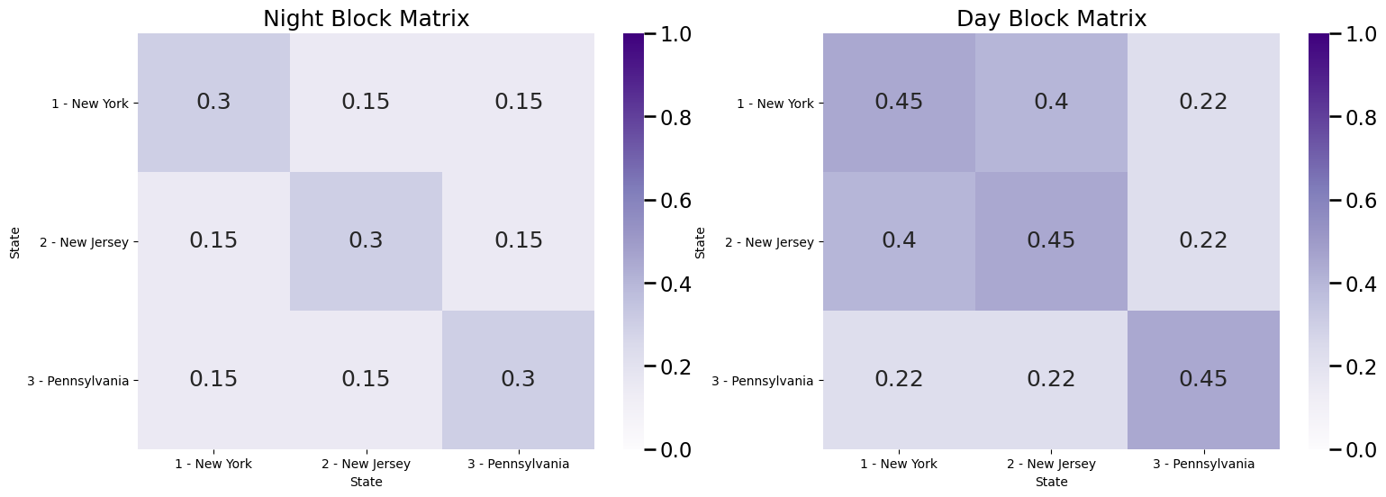
For a month, we measure the number of drivers who commute from one town to the other in a specified time window, and if more than \(1,000\) drivers regularly make this commute, we add an edge between the pair of towns. In general, we know that people tend to commute more frequently within their state, so the probabilities that an edge exists between a pair of towns in the same state exceeds the probabilities that an edge exists between a pair of towns which are not in the same state. Now, here’s the twist: we have measured the first network between 8 AM and 8 PM (covering the bulk of the work day), and the second network between 8 PM and 8 AM (covering the bulk of night time). We know that a lot of people in New Jersey tend to commute to new York for the work day, so we the probability of an edge existing between a New Jersey town and a New York town are higher during the day than the night. We don’t think that driving patterns themselves really change too much otherwise, but we do think that the probability of an edge existing is about \(50\%\) higher during the daytime. for all pairs of communities in the network. The block matrices look like this:

Bnight = np.array([[.3, .15, .15], [.15, .3, .15], [.15, .15, .3]])
Bday = Bnight*1.5  # day time block matarix is 50% more than night

# people tend to commute from New Jersey to New York during the day
Bday[0, 1] = .4; Bday[1,0] = .4

def plot_block(X, title="", blockname="State", blocktix=[0.5, 1.5, 2.5],
               blocklabs=["1 - New York", "2 - New Jersey", "3 - Pennsylvania"],
               ax=None):
    
    with sns.plotting_context("talk", font_scale=1):
        ax = sns.heatmap(X, cmap="Purples",
                        ax=ax, cbar_kws=dict(shrink=1), yticklabels=False,
                        xticklabels=False, vmin=0, vmax=1, annot=True)
        ax.set_title(title)
        cbar = ax.collections[0].colorbar
        ax.set(ylabel=blockname, xlabel=blockname)
        ax.set_yticks(blocktix)
        ax.set_yticklabels(blocklabs)
        ax.set_xticks(blocktix)
        ax.set_xticklabels(blocklabs)
        cbar.ax.set_frame_on(True)
    return

fig, axs = plt.subplots(1, 2, figsize=(18, 6))
plot_block(Bnight, title="Night Block Matrix", ax=axs[0])
plot_block(Bday, title="Day Block Matrix", ax=axs[1])
plt.show()

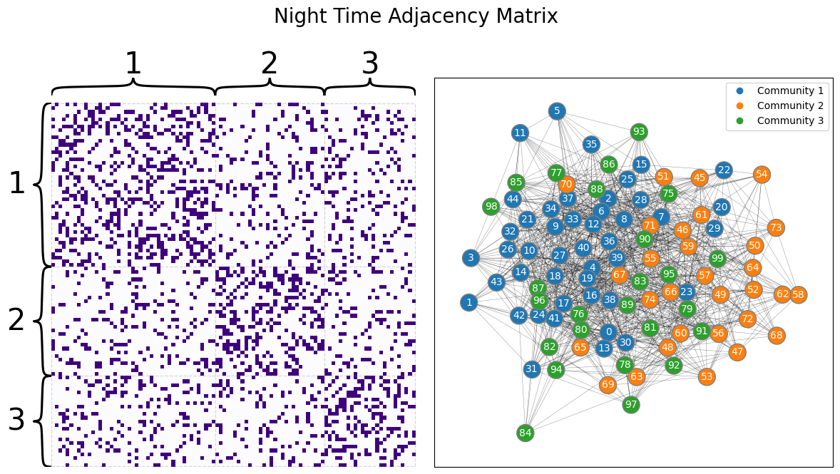
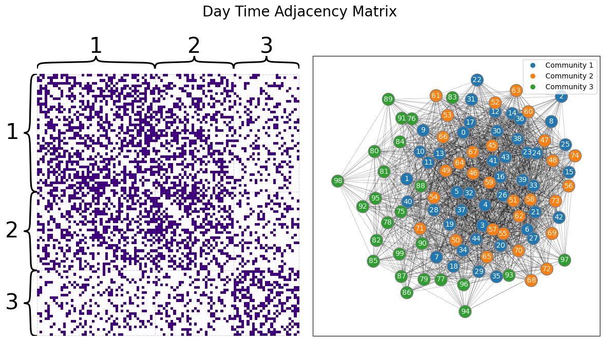
We then sample two networks with the above parameters, giving us the following two networks for the day and the night:

import graspologic as gp
from graspologic.simulations import sbm

Aday = sbm(ns, Bday)
Anight = sbm(ns, Bnight)

from graphbook_code import draw_multiplot

draw_multiplot(Anight, labels=list(z), title="Night Time Adjacency Matrix");
draw_multiplot(Aday, labels=list(z), title="Day Time Adjacency Matrix");

How can we ask whether the block matrices have similarities?

7.2.1. Testing whether the block matrices in an SBM are different

Based on what we learned above, we know ahead of time that the block matrices for the SBMs are different. However, how can we actually test this? Well, let’s start by being clear about what we mean by “different”. To make this a little big more mathemattical, we’ll introduce some new variables for the block matrices during the day time (\(B^{(d)}\)) and at night time (\(B^{(n)}\)) clearly. The block matrices are:

\[\begin{align*} B^{(d)} &= \begin{bmatrix} b^{(d)}_{11} & b^{(d)}_{12} & b^{(d)}_{13} \\ b^{(d)}_{21} & b^{(d)}_{22} & b^{(d)}_{23} \\ b^{(d)}_{31} & b^{(d)}_{32} & b^{(d)}_{33} \end{bmatrix}; \;\;\; B^{(n)} = \begin{bmatrix} b^{(n)}_{11} & b^{(n)}_{12} & b^{(n)}_{13} \\ b^{(n)}_{21} & b^{(n)}_{22} & b^{(n)}_{23} \\ b^{(n)}_{31} & b^{(n)}_{32} & b^{(n)}_{33} \end{bmatrix} \end{align*}\]

The hypothesis we want to test is the null hypothesis that the block matrices are the same, \(H_0: B^{(d)} = B^{(n)}\), against the alternative hypothesis that the block matrices are different, \(H_A: B^{(d)} \neq B^{(n)}\). For a matrix, remember that two matrices are equal if all of the entries are identical, and two matrices are unequal if at least one of the entries are unequal. We can rerformulate the null and alternative hypotheses with this logic.

For the null hypothesis, \(H_0: B^{(d)} = B^{(n)}\), the statement is therefore equivalent to saying that for all pairs of communities \(k\) and \(l\), \(b^{(d)}_{kl} = b^{(n)}_{kl}\). We will write each of these statements down as individual hypotheses for all pairs of communities, using the convention \(H_{0, kl}: b_{kl}^{(d)} = b^{(n)}_{kl}\). The null hypothesis \(H_0\) is therefore equivalent to saying that for every pair of communities \(k\) and \(l\), \(H_{0,kl}\) is true. For the alternative hypothesis, \(H_A: B^{(d)} \neq B^{(n)}\), the statement is therefore equivalent to saying that for at least one pair of communities \(k\) and \(l\), \(b^{(d)}_{kl} \neq b^{(n)}_{kl}\). We will write down each of these statements as well as individual hypotheses for all pairs of communities, using the convention \(H_{A, kl} : b_{kl}^{(d)} \neq b^{(n)}_{kl}\). The alternative hypothesis \(H_A\) is therefore equivalent to saying that for at least one pair of communities \(k\) and \(l\), that \(H_{A,kl}\) is true.

Now that we have broken a statement about two matrices down into numerous statements about two probabilities, we have almost completed our job. As it turns out, we have already seen the way we will test this, back in testing for differences in Section 6.2! Seeking to test whether a pair of block probabilities between communities \(k\) and \(l\) are the same, \(H_{0,kl}: b_{kl}^{(d)} = b_{kl}^{(n)}\), against whether the pair of block probabilities between communities \(k\) and \(l\) are different, \(H_{A, kl}: b_{kl}^{(d)} \neq b_{kl}^{(n)}\), is the two-sample testing problem Section 6.2.1.1.1! How did we address this problem before?

We used Fisher’s exact test! Remember that with Fisher’s exact test, for two probabilities that we want to compare, we construct the following contingency table for each pair of communities \(k\) and \(l\), with the entries:

	day	night
Number of edges	\(a\)	\(b\)
Number of non-edges	\(c\)	\(d\)

Where entry \(a\) is the total number of edges between nodes of community \(k\) with nodes of community \(l\) in the daytime network, and \(b\) is the total number of edges between nodes of community \(k\) with nodes of community \(l\) in the daytime network. The entry \(c\) the total number of edges between nodes of community \(k\) with nodes of community \(l\) in the daytime network that do not exist (the number of adjacencies in cluster one with an adjacency of zero), and the entry \(d\) is the total number of edges between nodes of community \(k\) with nodes of community \(l\) in the night time network that do not exist. We implement this using numpy and scipy, just like we did before, but this time for each pair of communities. To identify which adjacency matrix entries correspond to a given pair of communities, we use np.outer. Finally, we visualize the \(p\)-values of Fisher’s exact test for each pair of communities using a heatmap:

from scipy.stats import fisher_exact

K = 3
Pvals = np.empty((K, K))
# fill matrix with NaNs
Pvals[:] = np.nan

# get the indices of the upper triangle of Aday
upper_tri_idx = np.triu_indices(Aday.shape[0], k=1)
# create a boolean array that is nxn
upper_tri_mask = np.zeros(Aday.shape, dtype=bool)
# set indices which correspond to the upper triangle to True
upper_tri_mask[upper_tri_idx] = True

for k in range(0, K):
    for l in range(k, K):
        comm_mask = np.outer(z == (k+1), z == (l + 1))
        table = [[Aday[comm_mask & upper_tri_mask].sum(), Anight[comm_mask & upper_tri_mask].sum()],
                 [(Aday[comm_mask & upper_tri_mask] == 0).sum(), (Anight[comm_mask & upper_tri_mask] == 0).sum()]]
        Pvals[k,l] = fisher_exact(table)[1]

7.2.1.1. Adjusting for multiple comparisons

When we conducted our statistical tests above, you’ll notice that we run into the same problem that we had before: since we ran a bunch of tests, we have increased the familywise error rate. This means that we need to take care to handle the fact that we executed multiple comparisons. Again, we use Bonferroni-Holm adjustment from Section 6.3.3 for the \(p\)-values to visualize which community pairings are significantly different:

from statsmodels.stats.multitest import multipletests

# use bonferroni correction on p-values calculated from previous step
Pvals[~np.isnan(Pvals)] = multipletests(Pvals[~np.isnan(Pvals)], method='holm')[1]

# remove nans and replace with zeros temporarily
Pvals[np.isnan(Pvals)] = 0
# symmetrize since the network is undirected
Pvals = Pvals + Pvals.T + np.diag(np.diag(Pvals))

fig, ax = plt.subplots(1,1, figsize=(9, 6))
plot_block(Pvals, ax=ax, title="$p$-value matrix after Bonferrroni-Holm correction")

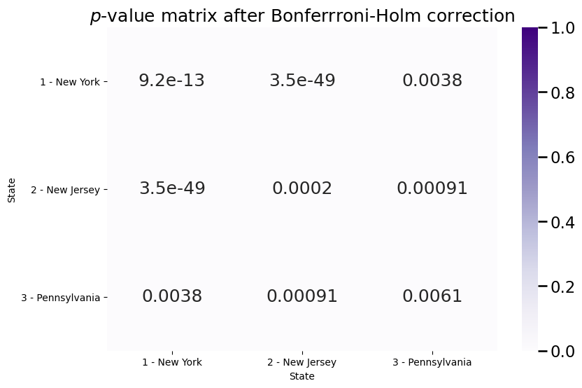
The \(p\)-values are all still less than \(\alpha=0.05\) after multiple hypothesis correction, so therefore, it seems like we have evidence to reject the null hypothesis that the block matrices are the same.

We still can’t answer our question about the block matrices themselves, because we have performed \(K \times K\) tests for each pair of communities, but need a single answer about \(H_0\) and \(H_A\). To achieve this, we need to combine the \(p\)-values, which can be done by using Tippett’s method for \(p\)-value combining [2]:

from scipy.stats import combine_pvalues
pval = combine_pvalues(Pvals.flatten(), method="tippett")[0]
print("p-value: {:3f}".format(pval))

p-value: 0.000000

The This can all be implemented using stochastic_block_test:

from pkg.stats import stochastic_block_test

stat, pvalue, misc = stochastic_block_test(
    Aday, Anight, labels1=z, labels2=z, method="fisher", combine_method="tippett"
)
print("p-value: {:.3f}".format(pvalue))

p-value: 0.000

The interpretation of a \(p\)-value below \(\alpha = 0.05\) is that we have evidence to reject the null hypothesis and conclude that the block matrices are different for day and night time.

7.2.2. Testing whether the block matrices in an SBM are multiples of one another

Back in Section 3.2.3.1 we learned about a useful summary statistic, known as the network density. If you remember, the network density was the quantity:

\[\begin{align*} density(A) &= \frac{2\sum_{j > i}a_{ij}}{n(n - 1)} \end{align*}\]

Which could be thought of as the “fraction” of edges which actually exist in a network, divided by the fraction of edges which could exist in a network. As it turns out, the network density plays an extremely large role ion virtually every property of networks which we estimate in machine learning, including the block matrices. However, when we talk about two block matrices being different, we might be trying to describe something more than just that their network densities are different.

For instance, in our example, we know that the probability of an edge existing between two cities is, in general, about \(50\%\) higher during the daytime compared to the night time. We don’t want to have our answer just be a product of the fact that there were just more edges in the daytime network. Rather, we want to find the topological difference between the two networks; that is, that the day time driving patterns between New Jersey and New York towns went above and beyond the \(50\%\) increase we otherwise had. For this reason, we revamp our hypothesis a little bit.

If you remember, our hypothesis that we ran above was the null hypothesis \(H_0: B^{(day)} = B^{(night)}\) that the two block matrices are the same against the alternative \(H_A: B^{(day)} \neq B^{(night)}\) that the block matrices differ. We will change this up a little bit. Now, our null hypothesis becomes \(H_0: B^{(day)} = a\cdot B^{(night)}\) that the two block matrices are the same up to a rescaling against \(H_A: B^{(day)} \neq a\cdot B^{(night)}\). How do we interpret this?

In this case, the value \(a\) is chosen to be the difference in the expected network densities between the day time and night time networks, the quantity \(a = \frac{p^{(day)}}{p^{(night)}}\). In practice, what we use is an estimate of this quantity, \(\hat a = \frac{\hat p^{(day)}}{\hat p^{(night)}}\), where \(\hat p^{(day)}\) is the network density of the day time network and \(\hat p^{(night)}\) is the network density of the night time network. Accepting the alternative hypothesis here means that the block matrices of the day and night time network are not simply multiples of each other.

We address this problem very similarly to above, instead using Fisher’s exact test for non-unity odds ratios from [3] and Chan2003Jan. We implement this using the bilateral connectome package [4], again showing the p-value matrix to visualize wiuch combinations of communities are substantially different:

n = np.sum(ns)

density_day = Aday[upper_tri_mask].sum()*2/(n*(n-1))
density_night = Anight[upper_tri_mask].sum()*2/(n*(n-1))

null_odds = density_day/density_night
stat, pvalue, misc = stochastic_block_test(
    Aday, Anight, labels1=z, labels2=z, method="fisher", combine_method="tippett",
    null_odds=null_odds
)
Pval_mtx = misc["uncorrected_pvalues"]

Bnight_adj = Bnight*null_odds

fig, axs = plt.subplots(1, 3, figsize=(27, 6))
plot_block(Bnight, title="Night Block Matrix", ax=axs[0])
plot_block(Bday/null_odds, title="Adjusted Day Block Matrix", ax=axs[1])
plot_block(Pval_mtx, title="adjusted P-value matrix, p-value={:.3f}".format(pvalue), ax=axs[2])
plt.show()

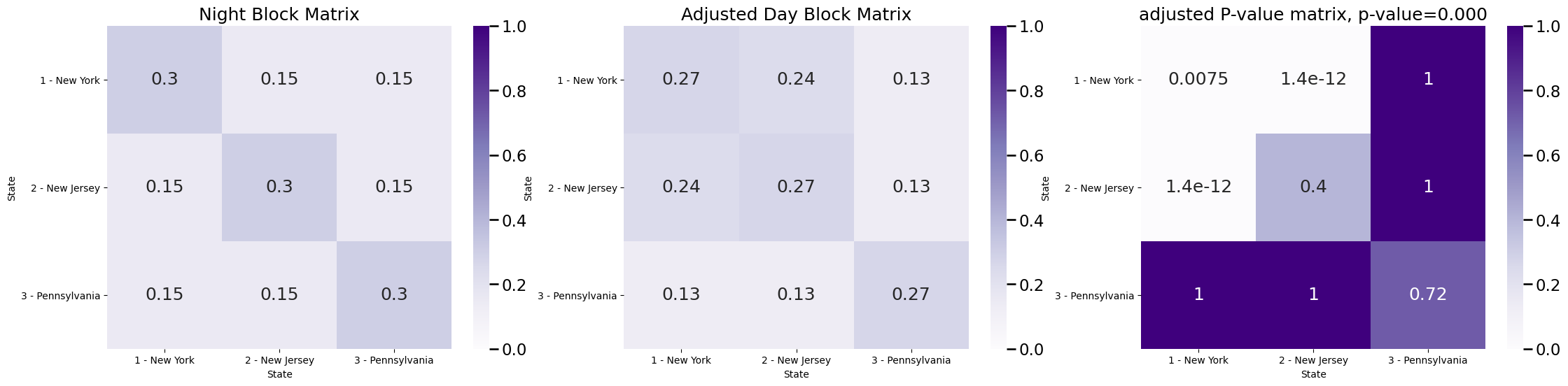
This shows that after we adjust the block matrix for changes in network density, the difference in the block probability for traveling New York and New Jersey is still significant. This means that the density-adjusted block matrices are different, since the \(p\)-value is less than \(\alpha = 0.05\). The interpretation here is that, after adjusting for density, we can still reject the null hypothesis in favor of the alternative that the block matrices for day and night time are still different, and that this difference can be accounted for by different traffic patterns between New York and New Jersey.

7.2.3. References

The paper at [1] discusses the theoretical properties of these procedures more in detail.

1

Benjamin D. Pedigo, Mike Powell, Eric W. Bridgeford, Michael Winding, Carey E. Priebe, and Joshua T. Vogelstein. Generative network modeling reveals quantitative definitions of bilateral symmetry exhibited by a whole insect brain connectome. bioRxiv, pages 2022.11.28.518219, November 2022. URL: https://doi.org/10.1101/2022.11.28.518219, arXiv:2022.11.28.518219.

2

L. H. C. Tippett. The Methods of Statistics. John Wiley and Sons, Hoboken, NJ, USA, January 1952. URL: https://www.amazon.com/Methods-Statistics-L-H-C-Tippett/dp/B019QJVM0W.

3

C. W. Dunnett and M. Gent. Significance testing to establish equivalence between treatments, with special reference to data in the form of 2X2 tables. Biometrics, 33(4):593–602, December 1977. URL: https://pubmed.ncbi.nlm.nih.gov/588654, arXiv:588654.

4

Benjamin Pedigo. neurodata/bilateral-connectome. February 2023. [Online; accessed 3. Feb. 2023]. URL: https://github.com/neurodata/bilateral-connectome.