4.1. Erdös-Rényi (ER) Random Networks#

We will start to learn about random networks with the simplest random network model. Consider a social network, with 50 students. Our network will have 50 nodes, where each node represents a single student in the network. Edges in the social network represent whether or not a pair of students are friends. What is the simplest way you could describe whether two people are friends?

In this case, the simplest possible thing to do would be to say, for any two students in our network, there is some probability (which we will call \(p\)) that describes how likely they are to be friends. In the below example, for the sake of argument, we will let \(p=0.3\). What does a sample from this network look like?

from graspologic.simulations import er_np

n = 50  # network with 50 nodes
p = 0.3  # probability of an edge existing is .3

# sample a single simple adjacency matrix from ER(50, .3)
A = er_np(n=n, p=p, directed=False, loops=False)

from graphbook_code import draw_multiplot
draw_multiplot(A, title="ER(0.3) Simulation");

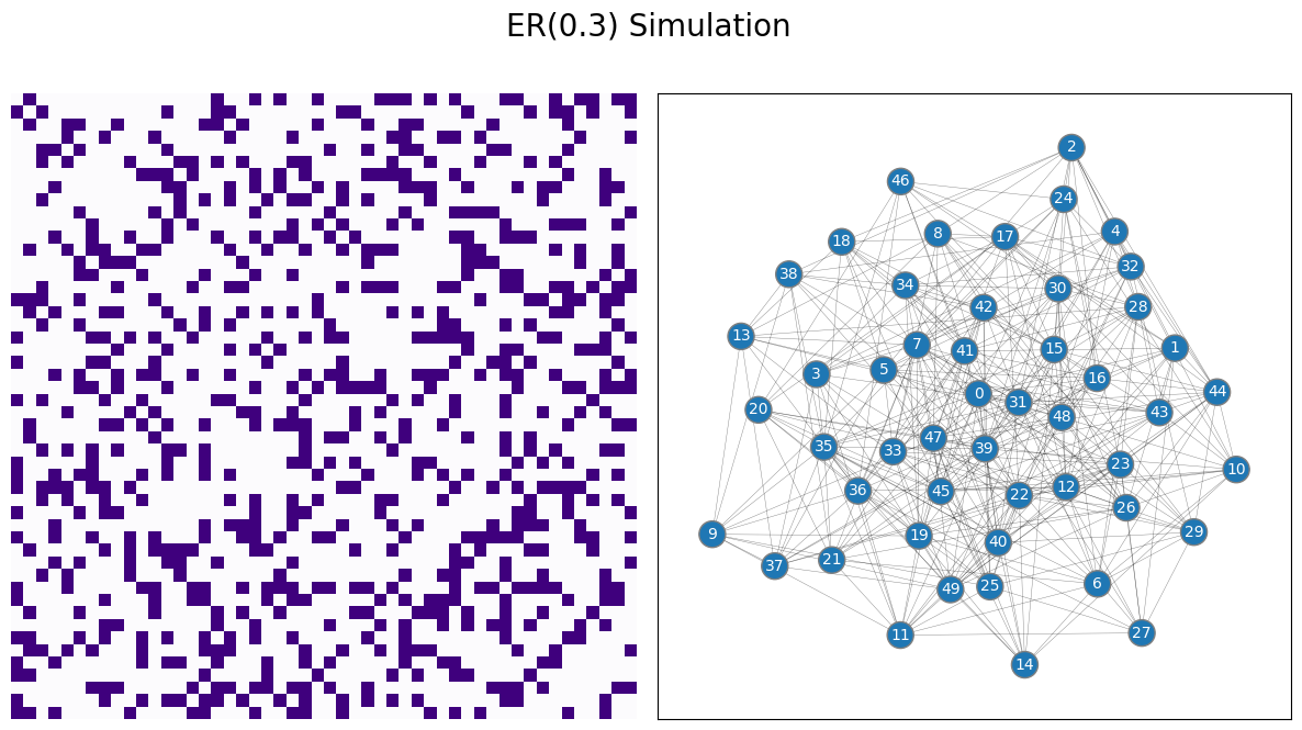
../../_images/single-network-models_ER_2_0.png

As we mentioned in the preface for this chapter, every statisical model in this book will come down to the coin flip model. In network machine learning, you get to see an adjacency matrix \(A\) whose entries \(a_{ij}\) are one if the students \(i\) and \(j\) are friends on the social networking site, and \(0\) if the students \(i\) and \(j\) are not friends on the social networking site. You have \(n\) students in total, so the adjacency matrix \(A\) is going to be \(n \times n\).

Now, let’s make the (seemingly) big leap to statistical modelling. When you have a coin, before you flip it, the outcome is either heads or tails, with some probability. We’ll denote this coin, for which we don’t know the outcome, by the letter \(\mathbf x\). The best way that we can describe this coin is not by heads and tails, but rather, by probabilities that it lands on heads or tails. For a coin, what we’d say is that a sample \(x\) (an outcome of a flip of the coin \(\mathbf x\)) is heads with probability \(p\) or tails with probability \(1-p\) (the coin can only land on heads or tails, so the probabilities must sum up to \(1\)). When specifying the statistical model, you don’t make any assumptions about the probabilities; you just specify that they are probabilities, and leave it at that. For a normal, fair coin, \(p\) would be \(0.5\), but we don’t even want to get that specific when we come up with a statistical model for a system.

Now, let’s rotate back to the network. Since \(A\) was an \(n \times n\) matrix, \(\mathbf A\) is an \(n \times n\) random matrix. The elements of \(\mathbf A\) will be given by the symbols \(\mathbf a_{ij}\), which means that each edge \(a_{ij}\) of \(A\) is a sample of the random edge \(\mathbf a_{ij}\). Just how do you describe this \(\mathbf a_{ij}\)? Remember that our samples \(a_{ij}\) are just \(0\)s and \(1\)s, which feels a lot like flipping a coin, doesn’t it? Did the coin land on heads, or did it land on tails? Are the two people \(i\) and \(j\) friends, or are they not friends? If you had a coin with some probability of landing on heads, you could describe \(a_{ij}\) as a sample of this coin flip. You could assume that a value of one is analogous to the coin landing on heads, and value of zero is analogous to the coin landing on tails. Perhaps you could even model the network using the same approach you took before with the coin flip. This is starting to go somewhere, so let’s continue with the analogies.

4.1.1. The Erdös Rényi random network is parametrized by the independent-edge probability#

This simple random network model is called the Erdös Rényi (ER) model, which was first described by [1] and [2]. The way you can think of an ER random network is that the edges depend only on a probability, \(p\), and each edge is totally independent of all other edges. You can think of this example as though a coin flip is performed, where the coin has a probability \(p\) of landing on heads, and \(1-p\) of landing on tails. For each edge in the network, you conceptually flip the coin, and if it lands on heads (with probability \(p\)), the edge exists, and if it lands on tails (with probability \(1-p\)) the edge does not exist. The meaning of independence is a little technical and goes a bit outside of the scope of this book, so we will leave it at a very high level as meaning that the outcome of particular coin flips do not impact the outcomes of other coin flips. This is not a very precise definition, but it will be plenty for our purposes. If \(\mathbf A\) is a random network which is \(ER_n(p)\) with \(n\) nodes and probability \(p\), we will say that \(\mathbf A\) is an \(ER_n(p)\) random network.

What part of this is the statistical model? The statistical model, here, is just the description of the system. all of the edges of the underlying random network, \(\mathbf A\), have a probability \(p\) of existing or not existing. This probability is the same for all edges. The edges are independent, and whether one edge exists does not impact whether any other edges exist. Again, the probability is left generic in the statistical model: it is just \(p\), which could be \(0.5\), \(0.7\), \(0.4\), really just any probability (a number between \(0\) and \(1\)). It’s really as simple as that!

4.1.2. How do you simulate samples of \(ER_n(p)\) random networks?#

This approach which you will use to describe random networks is called a generative model, which means that you have described an observable network sample \(A\) of the random network \(\mathbf A\) in terms of the parameters of \(\mathbf A\). In the case of the ER random networks, you have described \(\mathbf A\) in terms of the probability parameter, \(p\). Generative models are convenient in that you can easily adapt them to tell us exactly how to simulate samples of the underlying random network. The procedure below will produce for us a network \(A\), which has nodes and edges, where the underlying random network \(\mathbf A\) is an \(ER_n(p)\) random network:

Simulating a sample from an \(ER_n(p)\) random network

Choose a probability, \(p\), of an edge existing.
Obtain a weighted coin which has a probability \(p\) of landing on heads, and a probability \(1 - p\) of landing on tails. Note this probability \(p\) might differ from the “traditional” coin with a probability of landing on heads of approximately \(0.5\).
Flip the once for each possible edge \((i, j)\) between nodes \(i\) and \(j\) in the network. For a simple network, you will repeat the coin flip \(\binom n 2\) times.
For each coin flip which landed on heads, define that the corresponding edge exists, and define that the corresponding entry \(a_{ij}\) in the adjacency matrix is \(1\). For each coin flip which lands on tails, define that the corresponding edge does not exist, and define that \(a_{ij} = 0\).
The adjacency matrix you produce, \(A\), is a sample of an \(ER_n(p)\) random network.

4.1.3. When do you use an \(ER_n(p)\) Network?#

In practice, the \(ER_n(p)\) model seems like it might be a little too simple to be useful. Why would it ever be useful to think that the best you can do to describe our network is to say that connections exist with some probability? Does this miss a lot of useful questions you might want to answer? Fortunately, there are a number of ways in which the simplicity of the \(ER_n(p)\) model is useful. Given a probability and a number of nodes, you can easily describe the properties you would expect to see in a network if that network were ER. For instance, you know how many edges on average the nodes of an \(ER_n(p)\) random nework should have. You can reverse this idea, too: given a network you think might not be ER, you could check whether it’s different in some way from an \(ER_n(p)\) random network. It is often useful to start with the simplest random network models first when you are analyzing your network data, and only turning to more complicated network models when the need arises, because the types of network models you choose will directly determine the types of questions you can answer later on. For instance, if you see that half the nodes have a ton of edges (meaning, they have a high degree), and half don’t, you might be able to determine that the network is poorly described by an \(ER_n(p)\) random network. If this is the case, you might look for other models that could describe our network which are more complex.

In the next code block, you are going to sample a single \(ER_n(p)\) network with \(50\) nodes and an edge probability \(p\) of \(0.3\):

from graphbook_code import draw_multiplot
from graspologic.simulations import er_np

n = 10  # network with 50 nodes
p = 0.3  # probability of an edge existing is .3

# sample a single simple adjacency matrix from ER(50, .3)
A = er_np(n=n, p=p, directed=False, loops=False)

# and plot it
draw_multiplot(A, title="$ER_{10}(0.3)$ Simulation", xticklabels=10, yticklabels=10);

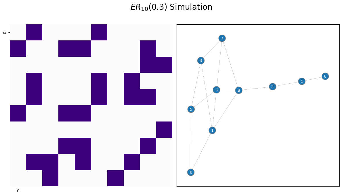
../../_images/single-network-models_ER_5_0.png

Above, you visualize the network using a heatmap. The dark squares indicate that an edge exists between a pair of nodes, and white squares indicate that an edge does not exist between a pair of nodes.

Next, let’s see what happens when you use a higher edge probability, like \(p=0.7\):

p = 0.7  # network has an edge probability of 0.7

# sample a single adjacency matrix from ER(50, 0.7)
A = er_np(n=n, p=p, directed=False, loops=False)

# and plot it
draw_multiplot(A, title="$ER_{10}(0.7)$ Simulation", xticklabels=10, yticklabels=10);

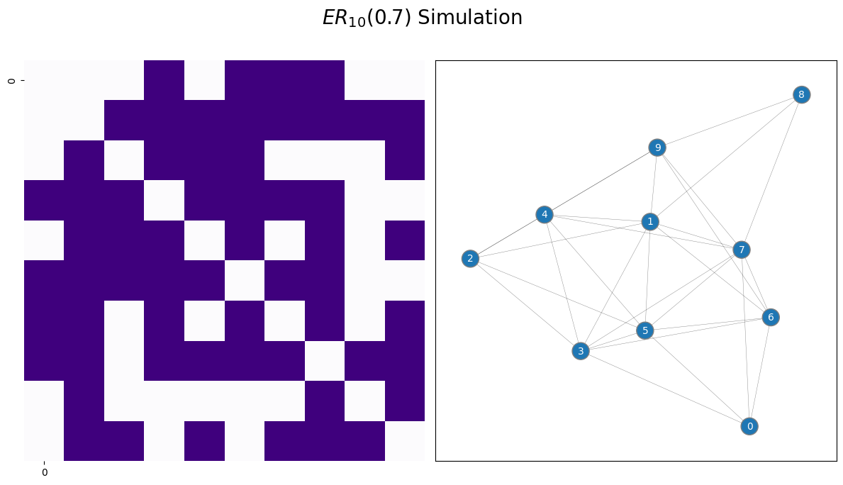
../../_images/single-network-models_ER_8_0.png

As the edge probability increases, the sampled adjacency matrix tends to indicate that there are more connections in the network. This is because there is a higher chance of an edge existing when \(p\) is larger.

4.1.4. Just how many networks are possible for a network with \(n\) nodes?#

As you’re going to become accustomed to, we’re going to boil this down again to coin flips. If you had one coin, there are two possible outcomes: either heads or tails. If you had two coins, the first coin could be heads or tails, and the second coin could be heads or tails. Let’s break this down by fixing the outcome of the first coin. If the first coin were heads, there are two possible outcomes for the second coin. If the first coin were tails, there are two possible outcomes for the second coin. This means that the total number of possible outcomes is the sum of the number of possible outcomes if the first coin is heads with the number of possible outcomes if the first coin were tails. This gives us that with two coins, you have four possible outcomes. When you add a third coin, you repeat this process again. If the first coin were heads, the second two coins could take any of four possible outcomes as you just learned. if the first coin were tails, the second two coins could also taake any of four possible outcomes. Therefore, with three coins, you have eight possible outcomes. As you continue this procedure, you quickly will realize that with \(x\) coin flips, you have \(2^x\) possible outcomes.

Remember in Section 3.2.3.1 when we were discussing the number of possible edges in a network, we determined that there are \(\frac{1}{2}n(n - 1)\) possible edges in a simple network, which we could represent using the notation \(\binom n 2\). In a realized network, each of these edges could exist or not exist, so there are again two possibilities just like the coin flips. Since edges existing or not existing boils down to a coin flip, the number of possible networks with \(n\) nodes is just \(2\) to the power of the number of coin flips that are performed in the network. Here, this is \(2^{\binom n 2}\). This quantity gets really big really fast! Let’s see just how fast below:

import numpy as np
from math import comb

ns = np.arange(2, 51)
nposs = np.array([comb(n, 2) for n in ns])*np.log10(2)

import seaborn as sns

ax = sns.lineplot(x=ns, y=nposs)
ax.set_title("")
ax.set_xlabel("Number of Nodes")
ax.set_ylabel("Number of Possible Networks (log scale)")
ax.set_yticks([50, 100, 150, 200, 250, 300, 350])
ax.set_yticklabels(["$10^{{{pow:d}}}$".format(pow=d) for d in [50, 100, 150, 200, 250, 300, 350]])
ax;

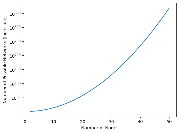
../../_images/single-network-models_ER_11_0.png

This is an enormous quantity! When \(n\) is just \(6\), the number of possible networks is \(2^{\binom 6 2} = 2^{6}\) which is over \(32,000\). When \(n\) is \(15\), the number of posssible networks balloons up to \(2^{\binom{15}{2}} = 2^{105}\) which is over \(10^{30}\). As the number of nodes increases, the number of possible network balloons really, really fast!

4.1.5. References#

If you want a deeper level of technical depth, please see the appendix Section 11.4.

1: P. Erdös and A. Rényi. On random graphs i. Publicationes Mathematicae Debrecen, 6:290, 1959.
2: E. N. Gilbert. Random Graphs. Ann. Math. Stat., 30(4):1141–1144, December 1959. doi:10.1214/aoms/1177706098.

Hands-on Network Machine Learning with Scikit-Learn and Graspologic

Erdös-Rényi (ER) Random Networks

Contents