11.3. Foundation#

To understand network models, it is crucial to understand the concept of a network as a random quantity, taking a probability distribution. We have a realization $A$, and we think that this realization is random in some way. Stated another way, we think that there exists a network-valued random variable $\mathbf A$ that governs the realizations we get to see. Since $\mathbf A$ is a random variable, we can describe it using a probability distribution. The distribution of the random network $\mathbf A$ is the function $Pr$ which assigns probabilities to every possible configuration that $\mathbf A$ could take. Notationally, we write that $\mathbf A \sim Pr$, which is read in words as “the random network $\mathbf A$ is distributed according to $Pr$.”

In the preceding description, we made a fairly substantial claim: $Pr$ assigns probabilities to every possible configuration that realizations of $\mathbf A$, denoted by $A$, could take. How many possibilities are there for a network with $n$ nodes? Let’s limit ourselves to simple networks: that is, $A$ takes values that are unweighted ($A$ is binary), undirected ($A$ is symmetric), and loopless ($A$ is hollow). In words, $\mathcal A_n$ is the set of all possible adjacency matrices $A$ that correspond to simple networks with $n$ nodes. Stated another way: every $A$ that is found in $\mathcal A$ is a binary $n \times n$ matrix ($A \in \{0, 1\}^{n \times n}$), $A$ is symmetric ($A = A^\top$), and $A$ is hollow ($diag(A) = 0$, or $A_{ii} = 0$ for all $i = 1,...,n$). We describe $\mathcal A_n$ as:

\[\begin{align*} \mathcal A_n = \left\{A : A \textrm{ is an $n \times n$ matrix with $0$s and $1$s}, A\textrm{ is symmetric}, A\textrm{ is hollow}\right\} \end{align*}\]

To summarize the statement that $Pr$ assigns probabilities to every possible configuration that realizations of $\mathbf A$ can take, we write that $Pr : \mathcal A_n \rightarrow [0, 1]$. This means that for any $A \in \mathcal A_n$ which is a possible realization of a random network $\mathbf A$, that $Pr(\mathbf A = A)$ is a probability (it takes a value between $0$ and $1$). If it is completely unambiguous what the random variable $\mathbf A$ refers to, we might abbreviate $Pr(\mathbf A = A)$ with $Pr(A)$. This statement can alternatively be read that the probability that the random variable $\mathbf A$ takes the value $A$ is $Pr(A)$. Finally, let’s address that question we had in the previous paragraph. How many possible adjacency matrices are in $\mathcal A_n$?

Let’s imagine what just one $A \in \mathcal A_n$ can look like. Note that each matrix $A$ has $n \times n = n^2$ possible entries, in total, since $A$ is an $n \times n$ matrix. There are $n$ possible self-loops for a network, but since $\mathbf A$ is simple, it is loopless. This means that we can subtract $n$ possible edges from $n^2$, leaving us with $n^2 - n = n(n-1)$ possible edges that might not be unconnected. If we think in terms of a realization $A$, this means that we are ignoring the diagonal entries $a_{ii}$, for all $i \in [n]$. Remember that a simple network is also undirected. In terms of the realization $A$, this means that for every pair $i$ and $j$, that $a_{ij} = a_{ji}$. If we were to learn about an entry in the upper triangle of $A$ where $a_{ij}$ is such that $j > i$, note that we have also learned what $a_{ji}$ is, too. This symmetry of $A$ means that of the $n(n-1)$ entries that are not on the diagonal of $A$, we would, in fact, “double count” the possible number of unique values that $A$ could have. This means that $A$ has a total of $\frac{1}{2}n(n - 1)$ possible entries which are free, which is equal to the expression $\binom{n}{2}$. Finally, note that for each entry of $A$, that the adjacency can take one of two possible values: $0$ or $1$. To write this down formally, for every possible edge which is randomly determined, we have two possible values that edge could take. Let’s think about building some intuition here:

If $A$ is $2 \times 2$, there are $\binom{2}{2} = 1$ unique entry of $A$, which takes one of $2$ values. There are $2$ possible ways that $A$ could look:

\[\begin{align*} \begin{bmatrix} 0 & 1 \\ 1 & 0 \end{bmatrix}\textrm{ or } \begin{bmatrix} 0 & 0 \\ 0 & 0 \end{bmatrix} \end{align*}\]

If $A$ is $3 \times 3$, there are $\binom{3}{2} = \frac{3 \times 2}{2} = 3$ unique entries of $A$, each of which takes one of $2$ values. There are $8$ possible ways that $A$ could look:

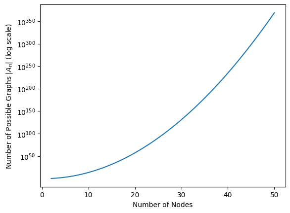
\[\begin{align*} &\begin{bmatrix} 0 & 1 & 1 \\ 1 & 0 & 1 \\ 1 & 1 & 0 \end{bmatrix}\textrm{ or } \begin{bmatrix} 0 & 1 & 0 \\ 1 & 0 & 1 \\ 0 & 1 & 0 \end{bmatrix}\textrm{ or } \begin{bmatrix} 0 & 0 & 1 \\ 0 & 0 & 1 \\ 1 & 1 & 0 \end{bmatrix} \textrm{ or }\\ &\begin{bmatrix} 0 & 1 & 1 \\ 1 & 0 & 0 \\ 1 & 0 & 0 \end{bmatrix}\textrm{ or } \begin{bmatrix} 0 & 0 & 1 \\ 0 & 0 & 0 \\ 1 & 0 & 0 \end{bmatrix}\textrm{ or } \begin{bmatrix} 0 & 0 & 0 \\ 0 & 0 & 1 \\ 0 & 1 & 0 \end{bmatrix}\textrm{ or }\\ &\begin{bmatrix} 0 & 1 & 0 \\ 1 & 0 & 0 \\ 0 & 0 & 0 \end{bmatrix}\textrm{ or } \begin{bmatrix} 0 & 0 & 0 \\ 0 & 0 & 0 \\ 0 & 0 & 0 \end{bmatrix} \end{align*}\]

How do we generalize this to an arbitrary choice of $n$? The answer is to use combinatorics. Basically, the approach is to look at each entry of $A$ which can take different values, and multiply the total number of possibilities by $2$ for every element which can take different values. Stated another way, if there are $2$ choices for each one of $x$ possible items, we have $2^x$ possible ways in which we could select those $x$ items. But we already know how many different elements there are in $A$, so we are ready to come up with an expression for the number. In total, there are $2^{\binom n 2}$ unique adjacency matrices in $\mathcal A_n$. Stated another way, the cardinality of $\mathcal A_n$, described by the expression $|\mathcal A_n|$, is $2^{\binom n 2}$. The cardinality here just means the number of elements that the set $\mathcal A_n$ contains. When $n$ is just $15$, note that $\left|\mathcal A_{15}\right| = 2^{\binom{15}{2}} = 2^{105}$, which when expressed as a power of $10$, is more than $10^{30}$ possible networks that can be realized with just $15$ nodes! As $n$ increases, how many unique possible networks are there? In the below figure, look at the value of $|\mathcal A_n| = 2^{\binom n 2}$ as a function of $n$. As we can see, as $n$ gets big, $|\mathcal A_n|$ grows really really fast!

import seaborn as sns
import numpy as np
from math import comb


n = np.arange(2, 51)
logAn = np.array([comb(ni, 2) for ni in n])*np.log10(2)

ax = sns.lineplot(x=n, y=logAn)
ax.set_title("")
ax.set_xlabel("Number of Nodes")
ax.set_ylabel("Number of Possible Graphs $|A_n|$ (log scale)")
ax.set_yticks([50, 100, 150, 200, 250, 300, 350])
ax.set_yticklabels(["$10^{{{pow:d}}}$".format(pow=d) for d in [50, 100, 150, 200, 250, 300, 350]])
ax;

So, now we know that we have probability distributions on networks, and a set $\mathcal A_n$ which defines all of the adjacency matrices that every probability distribution must assign a probability to. Now, just what is a network model? A network model is a set $\mathcal P$ of probability distributions on $\mathcal A_n$. Stated another way, we can describe $\mathcal P$ to be:

\[\begin{align*} \mathcal P &\subseteq \{Pr: Pr\textrm{ is a probability distribution on }\mathcal A_n\} \end{align*}\]

In general, we will simplify $\mathcal P$ through something called parametrization. We define $\Theta$ to be the set of all possible parameters of the random network model, and $\theta \in \Theta$ is a particular parameter choice that governs the parameters of a specific network-valued random variable $\mathbf A$. In this case, we will write $\mathcal P$ as the set:

\[\begin{align*} \mathcal P(\Theta) &= \left\{Pr_\theta : \theta \in \Theta\right\} \end{align*}\]

If $\mathbf A$ is a random network that follows a network model, we will write that $\mathbf A \sim Pr_\theta$, for some arbitrary set of parameters $\theta$.

If you are used to traditional univariate or multivariate statistical modelling, an extremely natural choice for when you have a discrete sample space (like $\mathcal A_n$, which is discrete because we can count it) would be to use a categorical model. In the categorical model, we would have a single parameter for all possible configurations of an $n$-node network; that is, $|\theta| = \left|\mathcal A_n\right| = 2^{\binom n 2}$. What is wrong with this model? The limitations are two-fold:

As we explained previously, when $n$ is just $15$, we would need over $10^{30}$ bits of storage just to define $\theta$. This amounts to more than $10^{8}$ zetabytes, which exceeds the storage capacity of the entire world.
With a single network observed (or really, any number of networks we could collect in the real world) we would never be able to get a reasonable estimate of $2^{\binom n 2}$ parameters for any reasonably non-trivial number of nodes $n$. For the case of one observed network $A$, an estimate of $\theta$ (referred to as $\hat\theta$) would simply be for $\hat\theta$ to have a $1$ in the entry corresponding to our observed network, and a $0$ everywhere else. Inferentially, this would imply that the network-valued random variable $\mathbf A$ which governs realizations $A$ is deterministic, even if this is not the case. Even if we collected potentially many observed networks, we would still (with very high probability) just get $\hat \theta$ as a series of point masses on the observed networks we see, and $0$s everywhere else. This would mean our parameter estimates $\hat\theta$ would not generalize to new observations at all, with high probability.

So, what are some more reasonable descriptions of $\mathcal P$? We explore some choices below. Particularly, we will be most interested in the independent-edge networks. These are the families of networks in which the generative procedure which governs the random networks assume that the edges of the network are generated independently. Statistical Independence is a property which greatly simplifies many of the modelling assumptions which are crucial for proper estimation and rigorous statistical inference, which we will learn more about in the later chapters.

11.3.1. Equivalence Classes#

In all of the below models, we will explore the concept of the probability equivalence class, or an equivalence class, for short. The probability is a function which in general, describes how effective a particular observation $A$ can be described by a random variable $\mathbf A$ with parameters $\theta$, written $\mathbf A \sim Pr_\theta$. The probability will be used to describe the probability $Pr_\theta(\mathbf A)$ of observing the realization $A$ if the underlying random variable $\mathbf A$ has parameters $\theta$. Why does this matter when it comes to equivalence classes? An equivalence class is a subset of the sample space $E \subseteq \mathcal A_n$, which has the following properties. Holding the parameters $\theta$ fixed:

If $A$ and $A'$ are members of the same equivalence class $E$ (written $A, A' \in E$), then $Pr_\theta(A) = Pr_\theta(A')$.
If $A$ and $A''$ are members of different equivalence classes; that is, $A \in E$ and $A'' \in E'$ where $E, E'$ are equivalence classes, then $Pr_\theta(A) \neq Pr_\theta(A'')$.
Using points 1 and 2, we can establish that if $E$ and $E'$ are two different equivalence classes, then $E \cap E' = \varnothing$. That is, the equivalence classes are mutually disjoint.
We can use the preceding properties to deduce that given the sample space $\mathcal A_n$ and a probability function $Pr_\theta$, we can define a partition of the sample space into equivalence classes $E_i$, where $i \in \mathcal I$ is an arbitrary indexing set. A partition of $\mathcal A_n$ is a sequence of sets which are mutually disjoint, and whose union is the whole space. That is, $\bigcup_{i \in \mathcal I} E_i = \mathcal A_n$.

We will see more below about how the equivalence classes come into play with network models, and in a later section, we will see their relevance to the estimation of the parameters $\theta$.

11.3.2. Independent-Edge Random Networks#

The below models are all special families of something called independent-edge random networks. An independent-edge random network is a network-valued random variable, in which the collection of edges are all independent. In words, this means that for every adjacency $\mathbf a_{ij}$ of the network-valued random variable $\mathbf A$, that $\mathbf a_{ij}$ is independent of $\mathbf a_{i'j'}$, any time that $(i,j) \neq (i',j')$. When the networks are simple, the easiest thing to do is to assume that each edge $(i,j)$ is connected with some probability (which might be different for each edge) $p_{ij}$. We use the $ij$ subscript to denote that this probability is not necessarily the same for each edge. This simple model can be described as $\mathbf a_{ij}$ has the distribution $Bern(p_{ij})$, for every $j > i$, and is independent of every other edge in $\mathbf A$. We only look at the entries $j > i$, since our networks are simple. This means that knowing a realization of $\mathbf a_{ij}$ also gives us the realizaaion of $\mathbf a_{ji}$ (and thus $\mathbf a_{ji}$ is a deterministic function of $\mathbf a_{ij}$). Further, we know that the random network is loopless, which means that every $\mathbf a_{ii} = 0$. We will call the matrix $P = (p_{ij})$ the probability matrix of the network-valued random variable $\mathbf A$. In general, we will see a common theme for the probabilities of a realization $A$ of a network-valued random variable $\mathbf A$, which is that it will greatly simplify our computation. Remember that if $\mathbf x$ and $\mathbf y$ are binary variables which are independent, that $Pr(\mathbf x = x, \mathbf y = y) = Pr(\mathbf x = x) Pr(\mathbf y = y)$. Using this fact:

\[\begin{align*} Pr(\mathbf A = A) &= Pr(\mathbf a_{11} = a_{11}, \mathbf a_{12} = a_{12}, ..., \mathbf a_{nn} = a_{nn}) \\ &= Pr(\mathbf a_{ij} = a_{ij} \text{ for all }j > i) \\ &= \prod_{j > i}Pr(\mathbf a_{ij} = a_{ij}), \;\;\;\;\textrm{Independence Assumption} \end{align*}\]

Next, we will use the fact that if a random variable $\mathbf a_{ij}$ has the Bernoulli distribution with probability $p_{ij}$, that $Pr(\mathbf a_{ij} = a_{ij}) = p_{ij}^{a_{ij}}(1 - p_{ij})^{1 - p_{ij}}$:

\[\begin{align*} Pr_\theta(A) &= \prod_{j > i}p_{ij}^{a_{ij}}(1 - p_{ij})^{1 - p_{ij}} \end{align*}\]

Now that we’ve specified a probability and a very generalizable model, we’ve learned the full story behind network models and are ready to skip to estimating parameters, right? Wrong! Unfortunately, if we tried too estimate anything about each $p_{ij}$ individually, we would obtain that $p_{ij} = a_{ij}$ if we only have one realization $A$. Even if we had many realizations of $\mathbf A$, this still would not be very interesting, since we have a lot of $p_{ij}$s to estimate, and we’ve ignored any sort of structural model that might give us deeper insight into $\mathbf A$. In the below sections, we will learn successively less restrictive (and hence, more expressive) assumptions about $p_{ij}$s, which will allow us to convey fairly complex random networks, but still enable us with plenty of intteresting things to learn about later on.

Hands-on Network Machine Learning with Scikit-Learn and Graspologic

Foundation

Contents

11.3. Foundation#

11.3.1. Equivalence Classes#

11.3.2. Independent-Edge Random Networks#