3.4. Regularization#

In practice, many networks you will encounter in network machine learning will not be simple networks. As we discussed in the preceding discussion, many of the techniques we discuss will be just fine to use with weighted networks. Unfortunately, real world networks are often extremely noisy, and so the analysis of one real world network might not generalize very well to a similar real world network. For this reason, we turn to regularization.

Regularization is the process by which you either:

Modify data for the purpose of mitigating overfitting due to idiosyncrasies of the observed data, and/or
Modify the function you are estimating due to the fragility of the function you estimating to idiosyncracies of the observed data.

In network machine learning, the first step of your analysis is to typically modify the network (or networks) themselves to allow better generalization of your statistical inference to new datasets. Later chapters, such as Section 5 and many areas of the Applications, will cover approaches in which you modify the function you are estimating.

For each of the following subsections, we’ll pose an example, a simulation, and code for how to implement the desired regularization approach. It is important to realize that you might use several of these techniques simultaneously in practice, or you might have a reason to use these techniques that go outside of our working examples.

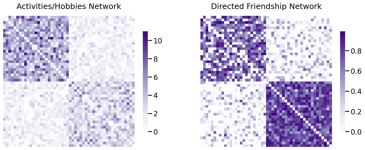
To start this section off, we’re going to introduce an example that’s going to be similar to those that you see in many future sections you see in this book. You have a group of \(50\) local students who attend a school in your area. The first \(25\) of the students polled are athletes, and the second \(25\) of the students polled are in marching band. You want to analyze how good of friends the students are, and to do so, you will use network machine learning. The nodes of the network will be the students. Next, we will describe how the two networks are collected:

Activity/Hobby Network: To collect the first network, you ask each student to select from a list of \(50\) school activities and outside hobbies that they enjoy. For a pair of students \(i\) and \(j\), the weight of their interest alignment will be a score between \(0\) and \(50\) indicating how many activities or hobbies that they have in common. We will refer to this network as the activity/hobby network. This network is obviously undirected, since if student \(i\) shares \(x\) activities or hobbies with student \(j\), then student \(j\) also shares \(x\) activities or hobbies with student \(i\). This network is weighted, since the score is between \(0\) and \(50\). Finally, this network is loopless, because it would not make sense to look at the activity/hobby alignment of a student with themself, since this number would be largely uninformative as every student would have perfect alignment of activities and hobbies with him or herself.
Friendship Network: To collect the second network, you ask each student to rate how good of friends they are with other students, on a scale from \(0\) to \(1\). A score of \(0\) means they are not friends with the student or do not know the student, and a score of \(1\) means the student is their best friend. We will refer to this network as the friendship network. This network is clearly directed, since two students may differ on their understanding of how good of friends they are. This network is weighted, since the score is between \(0\) and \(1\). Finally, this network is also loopless, because it would not make sense to ask somebody how good of friends they are with themself.

Our scientific question of interest is how well activities and hobbies align with perceived notions of friendship. You want to use the preceding networks to learn about a hypothetical third network, a network whose nodes are identical to the two networks above, but whose edges are whether the two individuals are friends (or not) on facebook. To answer this question, you have quite the job to do to make your networks better suited to the task! You begin by simulating some example data, shown below as adjacency matrix heatmaps:

from graspologic.simulations import sbm
import numpy as np

wtargsa = [[dict(n=50, p=.09), dict(n=50, p=.02)],
          [dict(n=50, p=.02), dict(n=50, p=.06)]]

wtargsf = [[dict(a=4, b=2), dict(a=2, b=5)],
          [dict(a=2, b=5), dict(a=6, b=2)]]

# activity network
A_activity = sbm(n=[25, 25], p=[[1,1], [1,1]], wt=np.random.binomial, wtargs=wtargsa, loops=False, directed=False)

# friend network
A_friend = sbm(n=[25, 25], p=[[.8, .4], [.4, 1]], wt=np.random.beta, wtargs=wtargsf, directed=True)

from graspologic.simulations import sbm
from matplotlib import pyplot as plt
from graphbook_code import heatmap

fig, axs = plt.subplots(1,2, figsize=(15, 6))

heatmap(A_activity, ax=axs[0], title="Activities/Hobbies Network")
heatmap(A_friend, ax=axs[1], title="Directed Friendship Network")
fig;

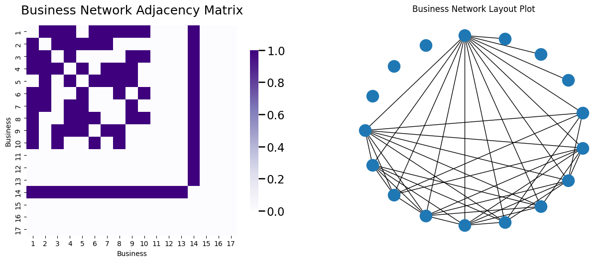
For good measure, we’ll also work with a third network which will have unique particularities from the preceding two, where we want to ask a question about only this network itself. This is going to be a business network, where the \(17\) nodes in the network are local businesses, and an edge exists between a pair of businesses if they have business dealings with one another (they buy or sell products from/with the company). Three of these businesses operate in total exclusion and do not have any edges. Three of these businesses only work with one other business. One businesses work with all of the non-excluded businesses. Let’s take a look at what this network looks like, with both a layout plot and an adjacency matrix.

from graspologic.simulations import er_np
n = 10
A_bus = er_np(n, 0.6)

# add pendants
n_pend = 3
A_bus = np.column_stack([np.row_stack([A_bus, np.zeros((n_pend, n))]), 
                         np.zeros((n + n_pend, n_pend))])

n = n + n_pend
# add pizza hut node
n_pizza = 1
A_bus = np.column_stack([np.row_stack([A_bus, np.ones((n_pizza, n))]), 
                         np.ones((n + n_pizza, n_pizza))])
n = n + n_pizza

# add isolates
n_iso = 3
A_bus = np.column_stack([np.row_stack([A_bus, np.zeros((n_iso, n))]), 
                         np.zeros((n + n_iso, n_iso))])
A_bus = A_bus - np.diag(np.diag(A_bus))
n = n + n_iso

import networkx as nx

fig, axs = plt.subplots(1,2, figsize=(15, 6))

node_names = [i for i in range(1, n+1)]
heatmap(A_bus, ax=axs[0], title="Business Network Adjacency Matrix", xticklabels=node_names, yticklabels=node_names);
axs[0].set_xlabel("Business"); axs[0].set_ylabel("Business");

G_bus = nx.from_numpy_matrix(A_bus)
node_pos = nx.shell_layout(G_bus)
nx.draw(G_bus, pos=node_pos, ax=axs[1])
axs[1].set_title("Business Network Layout Plot");

3.4.1. Node pruning#

Node pruning is a regularization technique in which you remove nodes for one reason or another. Typically, you will remove nodes due to some property about their degrees, or other properties (such as their connectedness with other nodes that you care about). These strategies are covered loosely in the book [1], and can be found in more computation-heavy network papers. Let’s take a look at some of the strategies.

3.4.1.1. Degree trimming removes nodes with unfavorable degrees#

In your business network, there are several nodes which tend to impart “strange” properties on downstream machine learning tasks. Some of these nodes, which include nodes with disproportionately high or low values, tend to yield numerical instability when you apply machine learning algorithms to them. By “numerical instability”, what we mean is that the the (few) connections that nodes with low degrees have are going to have a disproportionately large impact on the machine learning task we perform. For this reason, it may be advantageous to remove nodes whose degrees are much different from the other nodes in the network.

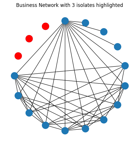
One special case of degree trimming is called removing isolates. An isolated node is a node which has a degree of \(0\), meaning that it is not connected to any other nodes in the network. In the network below, we’ve highlighted out the isolated nodes in red:

isolates = [14, 15, 16]
node_pos_isolates = {i: node_pos[node] for i, node in enumerate(isolates)}

A_bus_isolates = A_bus[14:17, 14:17]

G_bus_isolates = nx.from_numpy_matrix(A_bus_isolates)

fig, ax = plt.subplots(1,1, figsize=(6,6))
nx.draw(G_bus, pos=node_pos, ax=ax)
nx.draw(G_bus_isolates, pos=node_pos_isolates, node_color="red")
ax.set_title("Business Network with 3 isolates highlighted");

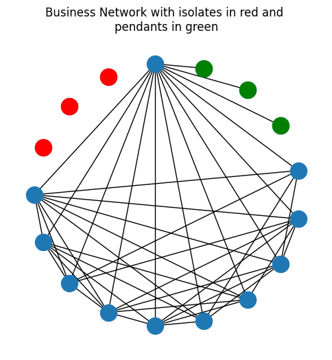
Another special case of degree trimming is called the removal of pendants. A pendant node is a node which has a degree of \(1\), meaning that it is only connected to one other node in the network. In the network below, we’ve now added the pendant nodes as well, in green:

pendants = [10, 11, 12]
node_pos_pendants = {i: node_pos[node] for i, node in enumerate(pendants)}

A_bus_pendants = A_bus[10:13, 10:13]

G_bus_pendants = nx.from_numpy_matrix(A_bus_pendants)

fig, ax = plt.subplots(1,1, figsize=(6,6))
nx.draw(G_bus, pos=node_pos, ax=ax)
nx.draw(G_bus_isolates, pos=node_pos_isolates, node_color="red")
nx.draw(G_bus_pendants, pos=node_pos_pendants, node_color="green")
ax.set_title("Business Network with isolates in red and \npendants in green");

You can remove isolates or pendants pretty simply. You simply need to compute the degree of each node in the network, and then retain the nodes with a degree above your chosen threshold. To remove isolates, you would pick this threshold to be \(0\) (retain nodes with non-zero degree), and to remove both pendants and isolates, you would pick this threshold to be \(1\) (retain nodes with a degree exceeding \(1\)). You can do this like follows:

def compute_degrees(A):
    # compute the degrees of the network A
    # since A is undirected, you can just sum
    # along an axis.
    return A.sum(axis=1)

def prune_low_degree(A, threshold=1):
    # remove nodes which have a degree under a given
    # threshold. For a simple network, threshold=0 removes isolates,
    # and threshold=1 removes pendants
    degrees = compute_degrees(A)
    non_prunes = degrees > threshold
    return A[np.where(non_prunes)[0],:][:,np.where(non_prunes)[0]]

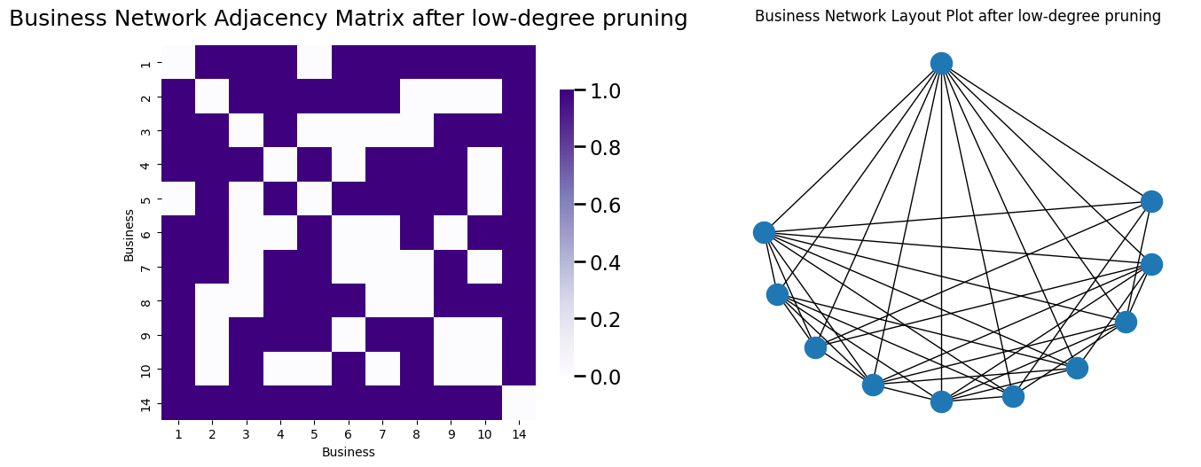
A_bus_lowpruned = prune_low_degree(A_bus)

high_degrees = [i for i in range(0, 10)] + [13]
node_names_lowpruned = [node_names[i] for i in high_degrees]
node_pos_lowpruned = {i : node_pos[j] for i, j in enumerate(high_degrees)}

G_bus_lowpruned = nx.from_numpy_matrix(A_bus_lowpruned)

fig, axs = plt.subplots(1,2, figsize=(15, 6))

node_names = [i for i in range(1, n+1)]
heatmap(A_bus_lowpruned, ax=axs[0], title="Business Network Adjacency Matrix after low-degree pruning", xticklabels=node_names_lowpruned,
        yticklabels=node_names_lowpruned);
axs[0].set_xlabel("Business"); axs[0].set_ylabel("Business");

nx.draw(G_bus_lowpruned, pos=node_pos_lowpruned, ax=axs[1])
axs[1].set_title("Business Network Layout Plot after low-degree pruning");

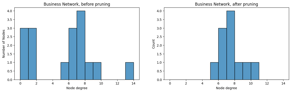
A useful way to determine whether you have isolates or pendants is to look at the degree distribution histogram of the network. The degree distribution histogram just shows a y axis of counts for a given range of possible x values. When the values you want a histogram for can only take a limited number of possible values, you might be able to get away with just looking at each possible value as its own x-axis point. Sometimes, when the values can take a large number of possible values, this might not be possible. You might have to bin similar values together to make the plot appreciable. The degree distribution, before and after removing pendants/isolates, looks like this:

degrees_before = compute_degrees(A_bus)
degrees_after = compute_degrees(A_bus_lowpruned)

from seaborn import histplot
fig, axs = plt.subplots(1,2, figsize=(15, 4))

ax = histplot(degrees_before, ax=axs[0], binwidth=1, binrange=(0, 14))
ax.set_xlabel("Node degree");
ax.set_ylabel("Number of Nodes");
ax.set_title("Business Network, before pruning");
ax = histplot(degrees_after, ax=axs[1], binwidth=1, binrange=(0, 14))
ax.set_xlabel("Node degree");
ax.set_title("Business Network, after pruning");

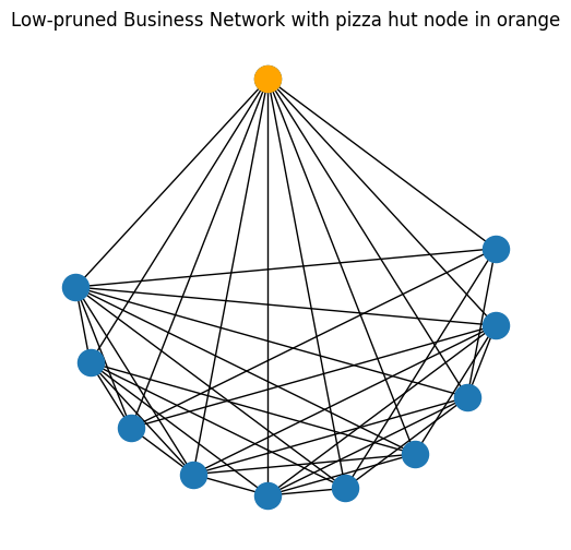
3.4.1.1.1. Removing pizza hut nodes#

On the other end of the spectrum, it is often useful to remove nodes which don’t really tell us anything about the network at all because they are just connected to everything. We call these nodes pizza hut nodes, because let’s face it, pizza hut can be delivered pretty much anywhere! After pruning, we actually created a pizza hut node, which we highlight here in orange:

pizza_node = [10]
node_pos_pizza = {i : node_pos_lowpruned[j] for i, j in enumerate(pizza_node)}
A_pizza = np.zeros((1,1))
G_pizza = nx.from_numpy_matrix(A_pizza)

fig, ax = plt.subplots(1,1, figsize=(6,6))
nx.draw(G_bus_lowpruned, pos=node_pos_lowpruned, ax=ax)
nx.draw(G_pizza, pos=node_pos_pizza, node_color="orange")
ax.set_title("Low-pruned Business Network with pizza hut node in orange");

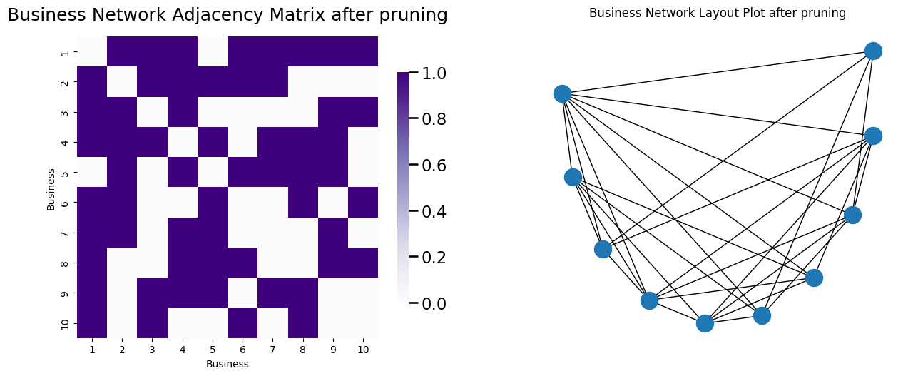
Pruning nodes with high degrees like pizza hut nodes is fairly easy. You can do this with a utility similar to the one you looked at above:

def prune_high_degree(A, threshold=0):
    # remove nodes which have a degree over a given
    # threshold. For a simple network, threshold=A.shape[0] - 1
    # removes any pizza hut node
    degrees = compute_degrees(A)
    non_prunes = degrees < threshold
    return A[np.where(non_prunes)[0],:][:,np.where(non_prunes)[0]]

A_bus_pruned = prune_high_degree(A_bus_lowpruned, threshold=A_bus_lowpruned.shape[0] - 1)

Which yields the network:

retained_nodes = [i for i in range(0, 10)]
node_names_retained = [node_names[i] for i in retained_nodes]
node_pos_retained = {i : node_pos[j] for i, j in enumerate(retained_nodes)}

G_bus_retained = nx.from_numpy_matrix(A_bus_pruned)

fig, axs = plt.subplots(1,2, figsize=(15, 6))

node_names = [i for i in range(1, 11)]
heatmap(A_bus_pruned, ax=axs[0], title="Business Network Adjacency Matrix after pruning", xticklabels=node_names_retained,
        yticklabels=node_names_retained);
axs[0].set_xlabel("Business"); axs[0].set_ylabel("Business");

nx.draw(G_bus_retained, pos=node_pos_retained, ax=axs[1])
axs[1].set_title("Business Network Layout Plot after pruning");

Again, you might want to look at the degree distribution plot to decide whether you want to prune nodes with high degrees.

3.4.1.2. The Largest Connected Component is the largest subnetwork of connected nodes#

Two sections ago in Section 3.2.4.1, you learned about computing the largest connected component. This is a node pruning technique, because it “throws out” all of the nodes other than the ones which are in the largest connected component. We would encourage you to go back through this example now if you have time, so that you will better associate it as a regularization technique in your brain.

3.4.2. Regularizing the Edges#

3.4.2.1. Symmetrizing the adjacency matrix gives us undirectedness#

If you wanted to learn from the friendship network about whether two people shared similar hobbies/activities, a reasonable first place to start might be to symmetrize the friendship adjacency matrix. The activity/hobby network is undirected, which means that if a student \(i\) is friends on facebook with student \(j\), then student \(j\) is also friends with student \(i\). On the other hand, as you learned above, the friendship network was directed. Since your question of interest is about an undirected network but the network you have is directed, it might be useful if you could take the directed friendship network and learn an undirected network from it. This relates directly to the concept of interpretability, in that you need to represent your friendship network in a form that will produce an answer for us about your facebook network which you can understand.

Another reason you might seek to symmetrize the friendship adjaceny matrix is that you might think that asymmetries that exist in the adjacency matrix are just noise. You might assume that the adjacency entries \(a_{ij}\) and \(a_{ji}\) relate to one another, so together they might be able to produce a single summary number that better summarizes their relationship all together.

As a final reason, you might think that the asymmetries are meaningful, but that they are not feasible to consider. Many statistical models for networks, and many techniques developed to analyze networks, might only have interpretations for undirected networks. This means that if you want to use these techniques, you might have to settle for making your network undirected first.

There are many other reasons you might want undirected networks, these are just a small subset of the reasons.

Jargon wise, remember that in a symmetric matrix (for an undirected network), \(a_{ij} = a_{ji}\), so in an asymmetric matrix (for a directed network), \(a_{ij} \neq a_{ji}\). To symmetrize the friendship network, what you want is a new adjacency value, which we will call \(w_{ij}\), which will be a function of \(a_{ij}\) and \(a_{ji}\). Then, you will construct a new adjacency matrix \(A'\), where each entry \(a_{ij}'\) and \(a_{ji}'\) are set equal to \(w_{ij}\). The little apostrophe just signifies that this is a potentially different value than either \(a_{ij}\) or \(a_{ji}\). Note that by construction, \(A'\) is in fact symmetric, because \(a_{ij}' = a_{ji}'\) due to how you built \(A'\).

3.4.2.1.1. Ignoring a “triangle” of the adjacency matrix#

The easiest way to symmetrize a network \(A\) is to just ignore part of it entirely. In the adjacency matrix \(A\), you will remember that you have an upper and a lower triangular part of the matrix:

\[\begin{align*} A &= \begin{bmatrix} a_{11} & \color{red}{a_{12}} & \color{red}{...} & \color{red}{a_{1n}} \\ \color{blue}{a_{21}} & \ddots & \color{red}{\ddots} & \color{red}{\vdots} \\ \color{blue}{\vdots} &\color{blue}{\ddots} &\ddots & \color{red}{a_{n-1, n}}\\ \color{blue}{a_{n1}} & \color{blue}{...} & \color{blue}{a_{n,n-1}} & a_{nn} \end{bmatrix}, \end{align*}\]

The entries which are listed in red are called the upper right triangle of the adjacency matrix above the diagonal. You will notice that for the entries in the upper right triangle of the adjacency matrix, \(a_{ij}\) is such that \(j\) is always greater than \(i\). Similarly, the entries which are listed in blue are called the lower left triangle of the adjacency matrix below the diagonal. In the lower left triangle, \(i\) is always greater than \(j\). These are called triangles because of the shape they make when you look at them in matrix form: notice, for instance, that in the upper right triangle, you have a triangle with three corners of values: \(a_{12}\), \(a_{1n}\), and \(a_{n-1, n}\).

So, how do you ignore a triangle all-together? Well, it’s really quite simple! We will visually show how to ignore the lower left triangle of the adjacency matrix. You start by forming a triangle matrix, \(\Delta\), as follows:

\[\begin{align*} \Delta &= \begin{bmatrix} 0 & \color{red}{a_{12}} & \color{red}{...} & \color{red}{a_{1n}} \\ \color{blue}{0} & \ddots & \color{red}{\ddots} & \color{red}{\vdots} \\ \color{blue}{\vdots} &\color{blue}{\ddots} &\ddots & \color{red}{a_{n-1, n}}\\ \color{blue}{0} & \color{blue}{...} & \color{blue}{0} & 0 \end{bmatrix}, \end{align*}\]

Notice that this matrix keeps all of the upper right triangle of the adjacency matrix above the diagonal the same as in the matrix \(A\), but replaces the lower left triangle of the adjacency matrix below the diagonal and the diagonal with \(0\)s. Notice that the transpose of \(\Delta\) is the matrix:

\[\begin{align*} \Delta^\top &= \begin{bmatrix} 0 & \color{blue}{0} & \color{blue}{...} &\color{blue}{0}\\ \color{red}{a_{12}}& \ddots & \color{blue}{\ddots} & \color{blue}{\vdots} \\ \color{red}{\vdots}&\color{red}{\ddots} & \ddots & \color{blue}{0} \\ \color{red}{a_{1n}}&\color{red}{...} &\color{red}{a_{n-1,n}} & 0 \end{bmatrix} \end{align*}\]

So when you add the two together, you get this:

\[\begin{align*} \Delta + \Delta^\top &= \begin{bmatrix} 0 & \color{red}{a_{12}} & \color{red}{...} & \color{red}{a_{1n}} \\ \color{red}{a_{12}} & \ddots & \color{red}{\ddots} & \color{red}{\vdots} \\ \color{red}{\vdots}&\color{red}{\ddots} &\ddots & \color{red}{a_{n-1, n}}\\ \color{red}{a_{1n}}&\color{red}{...} &\color{red}{a_{n-1,n}} & 0 \end{bmatrix}, \end{align*}\]

You’re almost there! You just need to add back the diagonal of \(A\), which you will do using the matrix \(diag(A)\) which has values \(diag(A)_{ii} = a_{ii}\), and \(diag(A)_{ij} = 0\) for any \(i \neq j\):

\[\begin{align*} A' &= \Delta + \Delta^\top + diag(A) = \begin{bmatrix} a_{11} & \color{red}{a_{12}} & \color{red}{...} & \color{red}{a_{1n}} \\ \color{red}{a_{12}} & \ddots & \color{red}{\ddots} & \color{red}{\vdots} \\ \color{red}{\vdots}&\color{red}{\ddots} &\ddots & \color{red}{a_{n-1, n}}\\ \color{red}{a_{1n}}&\color{red}{...} &\color{red}{a_{n-1,n}} & a_{nn} \end{bmatrix}, \end{align*}\]

Which leaves \(A'\) to be a matrix consisting only of entries which were in the upper right triangle of \(A\). \(A'\) is obviously symmetric, because \(a_{ij}' = a_{ji}'\) for all \(i\) and \(j\). Since the adjacency matrix is symmetric, the network \(A'\) represents is undirected.

3.4.2.1.1.1. When is “ignoring” a triangle appropriate?#

When you have an undirected network, it is often the case that the network will be stored only as a single “triangle”, since half of the matrix is redundant. Therefore, you can save potentially a lot of space by only storing half of it. So if you want the actual adjacency matrix, you need to “ignore” the uninformative triangle, and “retain” the informative one.

So what does this mean in terms of the network itself? This means that the network originally had edge weights \(a_{ij}\), where \(a_{ij}\) might not be equal to \(a_{ji}\). Let’s consider this in terms of the activity/hobby network. The activity/hobby network, which is undirected, perhaps has been stored in a representation where the entire lower-left triangle is just zeros, for space purposes. When you then upper-right symmetrize it, the network looks like this, using the graspologic function symmetrize with method="triu" (upper triangular symmetrization):

from graspologic.utils import symmetrize

# get only upper triangle
A_activity_uppertri = np.triu(A_activity)
# upper-triangle symmetrize the upper triangle
A_activity_triu_symmetrized = symmetrize(A_activity_uppertri, method="triu")

fig, axs = plt.subplots(1,2, figsize=(15, 6))

heatmap(A_activity_uppertri, ax=axs[0], title="Triangle of Activities/Hobbies Network")
heatmap(A_activity_triu_symmetrized, ax=axs[1], title="triu symmetrized triangle of Activity/Hobbies Network");

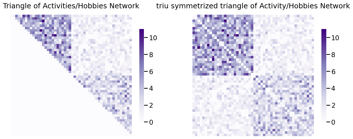
Likewise, if the network only had the lower triangle stored, you could do the same thing but with method="tril" to retain the lower triangle of the matrix.

3.4.2.1.2. Taking a function of the two values#

There are many other ways you use a function of \(a_{ij}\) and \(a_{ji}\) to get a symmetric matrix (and an undirected network). One is to just average. That is, you can let the matrix \(A'\) be the matrix with entries \(a'_{ij} = \frac{a_{ij} + a_{ji}}{2}\) for all \(i\) and \(j\). In matrix form, this operation looks like this:

\[\begin{align*} A' &= \frac{1}{2} (A + A^\top) \\ &= \frac{1}{2}\left(\begin{bmatrix} a_{11} & ... & a_{1n} \\ \vdots & \ddots & \vdots \\ a_{n1} & ... & a_{nn} \end{bmatrix} + \begin{bmatrix} a_{11} & ... & a_{n1} \\ \vdots & \ddots & \vdots \\ a_{1n} & ... & a_{nn} \end{bmatrix}\right)\\ &= \begin{bmatrix} \frac{1}{2}(a_{11} + a_{11}) & ... & \frac{1}{2}(a_{1n} + a_{n1}) \\ \vdots & \ddots & \vdots \\ \frac{1}{2} (a_{n1} + a_{1n}) & ... & \frac{1}{2}(a_{nn} + a_{nn}) \end{bmatrix} \\ &= \begin{bmatrix} a_{11} & ... & \frac{1}{2}(a_{1n} + a_{n1}) \\ \vdots & \ddots & \vdots \\ \frac{1}{2} (a_{n1} + a_{1n}) & ... & a_{nn} \end{bmatrix} \end{align*}\]

As you can see, for all of the entries, \(a'_{ij} = \frac{1}{2} (a_{ij} + a_{ji})\), and also \(a_{ji}' = \frac{1}{2}(a_{ji} + a_{ij})\). These quantities are the same, so \(a_{ij}' = a_{ji}'\), and \(A'\) is symmetric. As the adjacency matrix is symmetric, the network that \(A'\) represents is undirected.

Remember that the asymmetry in the friendship network means student \(i\) might perceive their friendship with student \(j\) as being stronger or weaker than student \(j\) perceived about student \(i\). What you did here was instead of just arbitrarily throwing one of those values away, you said that their friendship might be better indicated by averaging the two values. This produced for us a single friendship strength \(a_{ij}'\) where \(a_{ij}' = a_{ji}'\).

You can implement this in graspologic as follows:

# symmetrize with averaging
A_friend_avg_sym = symmetrize(A_friend, method="avg")

fig, axs = plt.subplots(1,2, figsize=(15, 6))

heatmap(A_friend, ax=axs[0], title="Directed Friendship Network")
heatmap(A_friend_avg_sym, ax=axs[1], title="Friendship Network, Symmetrized by Averaging")
fig;

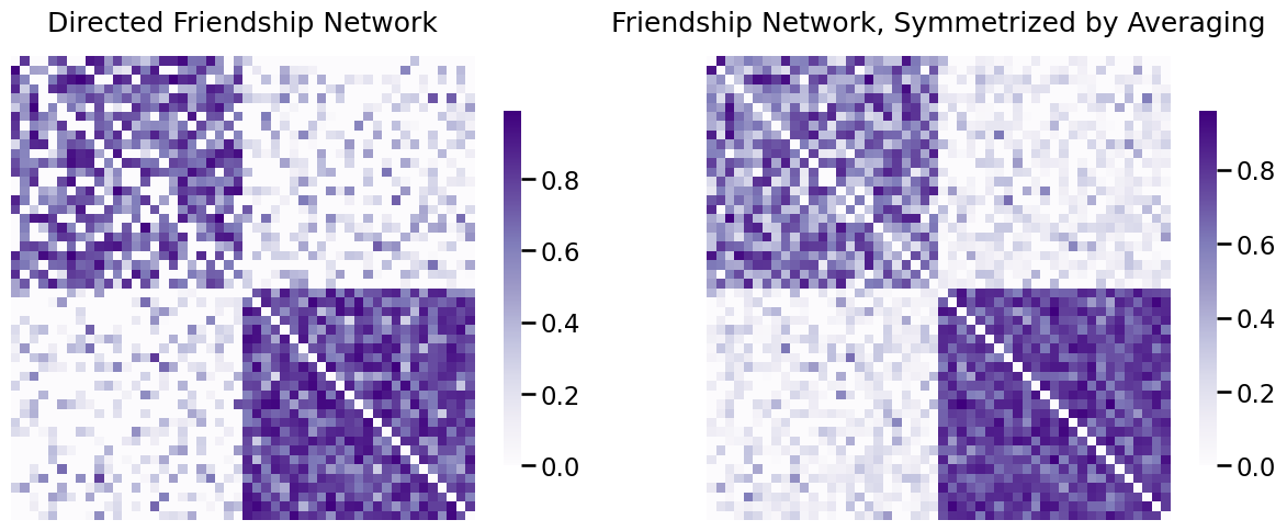
You will use the friendship network symmetrized by averaging in several of the below examples, which we will call the “undirected friendship network”.

3.4.2.2. Diagonal augmentation#

In your future works with network machine learning, you will come across numerous techniques which operate on adjacency matrices which are positive semi-definite. This word doesn’t need to mean a whole lot to you conceptually, but it has a big implication when you try to use algorithms on many of your networks. Remember that when you have a loopless network, a common practice in network science is to set the diagonal to zero. What this does is it leads to your adjacency matrices being indefinite (which means, not positive semi-definite). For our purposes, this means that many network machine learning techniques simply cannot operate on these adjacency matrices. However, as we mentioned before, these entries are not actually zero, but simply do not exist and you just didn’t have a better way to represent them. Or do we?

Diagonal augmentation is a procedure for imputing the diagonals of adjacency matrices for loopless networks. This gives us “placeholder” values that do not cause this issue of indefiniteness, and allow your network machine learning techniques to still work. Remember that for a simple network, the adjacency matrix will look like this:

\[\begin{align*} A &= \begin{bmatrix} 0 & a_{12} & ... & a_{1n} \\ a_{21}& \ddots & & \vdots \\ \vdots & & \ddots & a_{n-1, n} \\ a_{n1} &...& a_{n, n-1} & 0 \end{bmatrix} \end{align*}\]

What you do is impute the diagonal entries using the fraction of possible edges which exist for each node. This quantity is simply the node degree \(d_i\) (the number of edges which exist for node \(i\)) divided by the number of possible edges node \(i\) could have (which would be node \(i\) connected to each of the other \(n-1\) nodes). Remembering that the degree matrix \(D\) is the matrix whose diagonal entries are the degrees of each node, the diagonal-augmented adjacency matrix is given by:

\[\begin{align*} A' &= A + \frac{1}{n-1}D = \begin{bmatrix} \frac{d_1}{n-1} & a_{12} & ... & a_{1n} \\ a_{21}& \ddots & & \vdots \\ \vdots & & \ddots & a_{n-1, n} \\ a_{n1} &...& a_{n, n-1} & \frac{d_n}{n-1} \end{bmatrix} \end{align*}\]

When the matrices are directed or weighted, the computation is a little different, but fortunately graspologic will handle this for us. Let’s see how you would apply this to the directed friendship network:

from graspologic.utils import augment_diagonal

A_friend_aug = augment_diagonal(A_friend)

fig, axs = plt.subplots(1,3, figsize=(20, 6))

heatmap(A_friend, ax=axs[0], title="Directed Friendship Network, A")
heatmap(A_friend_aug, ax=axs[1], title="With Diagonal Augmentation, A'")
heatmap(A_friend_aug-A_friend, ax=axs[2], title="A' - A")
fig;

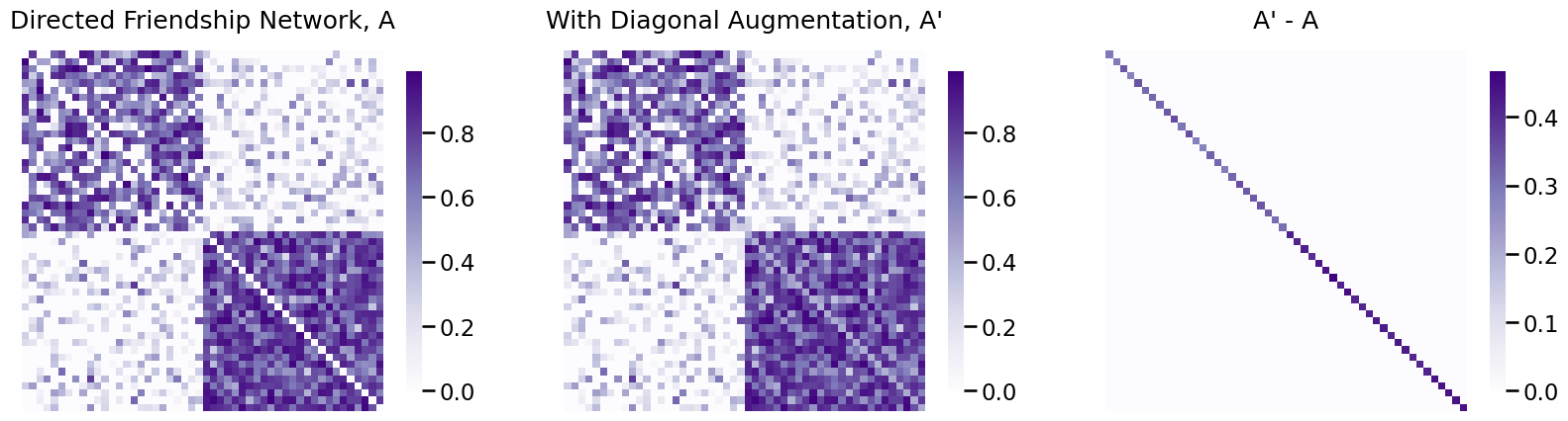
As you can see, the diagonal-augmented friendship network and the original directed friendship network differ only in that the diagonals of the diagonal-augmented friendship network are non-zero.

3.4.2.3. Regularizing edge weights#

As you are probably aware, in all of machine learning, you are always concerned with the bias/variance tradeoff. The bias/variance tradeoff is an unfortunate side-effect that concerns how well a learning technique will generalize to new datasets [1].

Bias is an error from erroneous assumptions you make about the system that you are learning about. For instance, if you have a friendship network, you might make simplifying assumptions, such as an assumption that two athletes frorm different sports have an equally likely chance of being friends with a member of the band. This might be flat out false, as band members might be selectively better friends with athletes depending on which sports they play.
On the other hand, the variance is the degree to which the an estimate of a task will change when given new data. An assumption that if a player is a football player he has a higher chance of being friends with a band member might make sense given that the band performs at football games.

The “trade-off” is that these two factors tend to be somewhat at odds, in that raising the bias tends to lower the variance, and vice-versa:

High bias, but low variance: Whereas a lower variance model might be better suited to the situation where the data you expect to see is noisy, it might not as faithfully represent the underlying dynamics you think the network possesses. A low variance model might ignore that athletes might have a different chance of being friends with a band member based on their sport all together. This means that while you won’t get the student relationships correct, you might still be able to get a reasonable estimate that you think is not due to overfitting. In this case, you’ve smoothed away signal from the data at the expense of avoiding noise.
Low bias, but high variance: Whereas a low bias model might more faithfully model true relationships in your training data, it might fit your training data a little too well. Fitting the training data too well is a problem known as overfitting. If you only had three football team members and tried to assume that football players were better friends with band members, you might not be able to well approximate this relationship because of how few individuals you have who reflect this situation.

Here, we show several strategies to reduce the variance (but, add bias) due to edge weight noise in network machine learning.

3.4.2.3.1. Sparsification of the network#

The procedure of sparsification is one in which we take a network, and we remove edges from it, which is described by [3] and [4]. Remember that removing edges, in terms of the adjacency matrix, is analogous to setting the corresponding adjacencies to zero. A matrix with many entries of zero is called a sparse matrix. So, the reason we call the removal of the edges from a network sparsification is that we are producing a network with a sparse adjacency matrix.

Sparsification is a general class of edge regularization techniques, and includes many flavors. Here, we discuss a few of them. In network sparsification, we will often pick some property of the network (such as, a particular edge weight) and remove edges in an attempt to preserve something about this particular property.

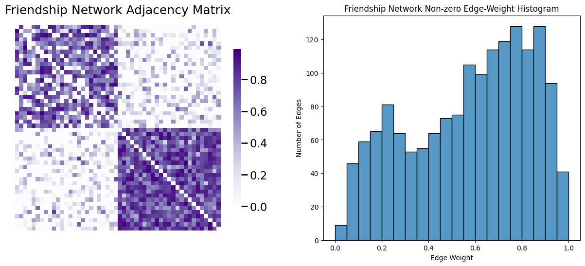
A useful tool to study for how, exactly, you might want to go about sparsifying the network is called the edge-weight distribution of your network sample. The edge-weight distribution of the network sample are the particular values that the edge weights of the network take. The most common way to visualize the edge-weight distribution is an edge-weight histogram. This is very similar to the node-degree histogram you worked with above, but instead of node degrees, you look at the edge-weights. Let’s take a look at the friendship network, and then take a look at its edge-weight distribution. Remember that the friendship network is undirected, so we need to remove its diagonal elements before we visualize the edge-weight distribution. We’ll also remove edges with zero-weights for visualization purposes:

# create a mask that is True for the non-diagonal edges
non_diag_idx = np.where(~np.eye(A_friend.shape[0], dtype=bool))
A_friend_nondiag_ew = A_friend[non_diag_idx].flatten()
# get the non-zero edge weights
A_friend_nondiag_nz_ew = A_friend_nondiag_ew[A_friend_nondiag_ew > 0]

fig, axs = plt.subplots(1,2, figsize=(15, 6))
heatmap(A_friend, ax=axs[0], title="Friendship Network Adjacency Matrix")
ax = histplot(A_friend_nondiag_nz_ew, ax=axs[1], bins=20, binrange=(0, 1))
ax.set_xlabel("Edge Weight");
ax.set_ylabel("Number of Edges");
ax.set_title("Friendship Network Non-zero Edge-Weight Histogram");

3.4.2.3.1.1. Truncation removes the smallest edges#

The simplest way to reduce the variance due to edge weight noise is called edge truncation. Edge truncation is a process by which you choose some threshold value \(\tau\), and remove all of the weights which are smaller than \(\tau\) but retain the weights that are bigger than \(\tau\). For edges that are equal to \(\tau\), what you’ll want to do depends on the strategy you are employing.

So, how is \(\tau\) typically chosen? There are a few ways, but it’s usually one of the below two:

Choose \(\tau\) arbitrarily: after looking at your network and doing some preliminary visualizations, you might determine that your edge weights tend to be “multi-modal”. This means that when you look at the edge-weight distribution, you see multiple “clusters” of edge weight bins which are larger, or smaller. For a lot of networks, these small edges might be very noise induced; that is, the small edges might just spuriously be close to, but not quite, zero, due to errors in your measuring process. When the edge weights are really tiny, you might think that these noisy edges are better off just not existing.
Choose \(\tau\) based on a particular quantile: A quantile is a percentile divided by \(100\). In this strategy, you identify a target quantile of the edge-weight distribution. What this means is that you are selecting the lowest fraction of the edge-weights (where that fraction is the quantile that you choose) and setting these edges to \(0\), and selecting the remaining edges are left unchanged. If you select a quantile of \(0.5\), this means that you take the smallest \(50\%\) of edges and set them to zero, and the largest \(50\%\) of edges and retain their initial value. This is called truncation because you are taking the edge-weight distribution, and truncating (cutting it off) below the value \(\tau\). Let’s see how this works in practice.

With respect to what to do with edges that are equal to \(\tau\), when you choose a threshold arbitrarily, you can do whatever you want with them, as long as you are consistent if you have multiple networks you are truncating. What we mean by this is that you can select to remove edges less than or equal to this threshold, or retain edge weights greater than or equal to the threshold. When you truncate on the basis of a quantile, however, this is not quite the case. You will want to remove all the edges below \(\tau\), and truncate away the remaining edges equal to \(\tau\) at random until you have truncated the desired fraction of edges in total.

In the edge-weight histogram, you can notice two “peaks” to the non-zero edge-weights:

fig, ax = plt.subplots(1,1, figsize=(8, 4))
ax = histplot(A_friend_nondiag_nz_ew, ax=ax, bins=20)
ax.set_xlabel("Edge Weight");
ax.set_ylabel("Number of Edges");
ax.set_title("Friendship Network Non-zero Edge-Weight Histogram");
ax.annotate("Small Peak", xytext=(.15, 110), xy=(.22, 80), color="red", arrowprops={"arrowstyle": "->", "color": "red", "lw": 2})
ax.annotate("Larger Peak", xytext=(.5, 120), xy=(.7, 140), color="red", arrowprops={"arrowstyle": "->", "color": "red", "lw": 2})
ax.axvline(x=0.4, ymin=0, ymax=140, color="red")
ax.annotate("$\\tau = 0.4$", xytext=(.25, 80), xy=(.4, 80), color="red", arrowprops={"arrowstyle": "->", "color": "red", "lw": 2});

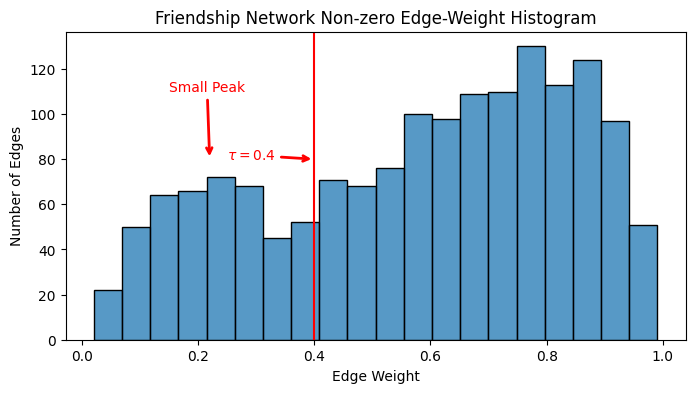
If you think that the smaller peak edge-weights are spurious/noise, you might want to threshold somewhere in between the smaller and the larger peaks, like near \(0.4\), which is highlighted above. First, we’ll truncate the edge-weight distribution at \(0.4\):

def truncate_network(A, threshold):
    A_cp = np.copy(A)
    A_cp[A_cp <= threshold] = 0
    return A_cp

tau = 0.4
A_friend_trunc = truncate_network(A_friend, threshold=tau)

Next, we’ll look at the adjacency matrix and the edge-weight distribution before/after truncation:

fig, axs = plt.subplots(1,2, figsize=(15, 6))
heatmap(A_friend, ax=axs[0], title="Friendship Network Adjacency Matrix")
heatmap(A_friend_trunc, ax=axs[1], title="Friendship Network Adjacency After Truncation");

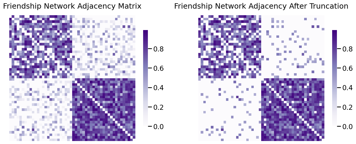
As you can see, a lot of the edges in the upper right and upper left, which were previously small, are now zero. This is reflected in the edge-weighte distribution:

A_friend_trunc_nz_nd_ew = A_friend_trunc[np.where(
    np.logical_and(~np.eye(A_friend_trunc.shape[0], dtype=bool),
                  A_friend_trunc > 0))].flatten()

fig, ax = plt.subplots(1,2, figsize=(15, 4))
histplot(A_friend_nondiag_nz_ew, ax=ax[0], bins=20, binrange=(0, 1))
ax[0].set_xlabel("Edge Weight");
ax[0].set_ylabel("Number of Edges");
ax[0].set_title("Friendship Network Non-zero Edge-Weight Histogram");
ax[0].annotate("Small Peak", xytext=(.15, 110), xy=(.22, 80), color="red", arrowprops={"arrowstyle": "->", "color": "red", "lw": 2})
ax[0].annotate("Larger Peak", xytext=(.5, 120), xy=(.7, 140), color="red", arrowprops={"arrowstyle": "->", "color": "red", "lw": 2})
ax[0].axvline(x=0.4, ymin=0, ymax=140, color="red")
ax[0].annotate("$\\tau = 0.4$", xytext=(.25, 80), xy=(.4, 80), color="red", arrowprops={"arrowstyle": "->", "color": "red", "lw": 2});


histplot(A_friend_trunc_nz_nd_ew, ax=ax[1], bins=20, binrange=(0, 1));
ax[1].set_xlabel("Edge Weight");
ax[1].set_ylabel("");
ax[1].set_title("Truncated Friendship Network Non-zero Edge-Weight Histogram");
ax[1].annotate("Larger Peak", xytext=(.5, 120), xy=(.7, 140), color="red", arrowprops={"arrowstyle": "->", "color": "red", "lw": 2})
ax[1].axvline(x=0.4, ymin=0, ymax=140, color="red")
ax[1].annotate("$\\tau = 0.4$", xytext=(.25, 80), xy=(.4, 80), color="red", arrowprops={"arrowstyle": "->", "color": "red", "lw": 2});

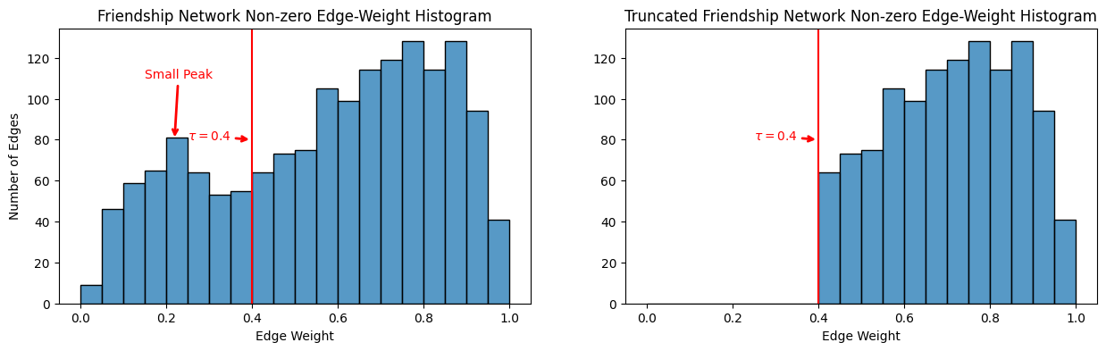
As you can see, all of the edges with weights less than \(\tau = 0.4\) have been truncated away.

A slight caveat to this procedure we learned about above for truncation is that, if you use the quantile approach and the network is undirected, you need to exclude one triangle of the network to obtain the appropriate quantile. We’ll see this more in the example on thresholding below.

3.4.2.3.1.2. Thresholding converts weighted networks to unweighted networks#

Closely related to truncation is the process of thresholding. Like truncation, you begin with a threshold \(\tau\), which is usually chosen arbitrarily or based on a quantile, like for truncation. However, there is one key difference: when you threshold a network, you set the edges below \(\tau\) to zero, and the edges greater than \(\tau\) to one. This has the effect of taking a weighted network, and effectively transforming it into an undirected network.

We will show how to use the quantile approach to thresholding, with the activity/hobby network. You will threshold by choosing \(\tau\) such that \(\tau\) is the value which is the \(0.5\) quantile, or the \(50\) percentile, of the edge-weight distribution. Remember as you learned in the preceding section, that if the network itself is loopless, the diagonal entries simply do not exist; \(0\) is simply a commonly used placeholder. For this reason, when you compute quantiles of edge-weights, you need to exclude the diagonal if the network is loopless.

Further, since this network is undirected, you also need to restrict your attention to one triangle of the corresponding adjacency matrix. We choose the upper-right triangle arbitrarily, as the adjacency matrix’s symmetry means the upper-right triangle and lower-right triangle have identical edge-weight distributions.

# find the indices which are in the upper triangle and not in the diagonal
upper_tri_non_diag_idx = np.where(np.triu(np.ones(A_activity.shape), k=1).astype(bool))
q = 0.5  # desired quantile is 0.5, or 50 percentile
tau = np.quantile(A_activity[upper_tri_non_diag_idx], q=q)

fig, axs = plt.subplots(1,1, figsize=(12, 5))
ax = histplot(A_activity[upper_tri_non_diag_idx].flatten(), ax=axs, bins=10)
ax.set_xlabel("Edge Weight");
ax.set_ylabel("Number of Edges");
ax.set_title("Activity/Hobby Network Off-Diagonal Edge-Weight Distribution");
ax.axvline(tau, color="red", linestyle="solid", linewidth=2)
plt.text(tau + .03, 250, "0.5 quantile, $\\tau = {:.3f}$".format(tau), fontsize=14, color="red");

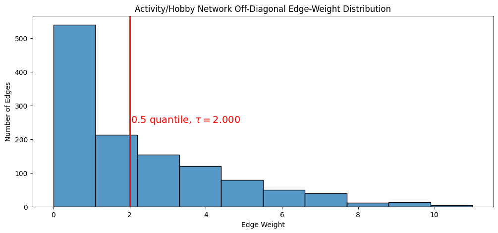
The \(0.5\) quantile, it turns out, is about \(2\). This is because about \(50\%\) of the edges are less than this threshold, and about \(50\%\) of the edges are greater than this threshold. We can see that the number of edges less than or equal to tau, and greater than tau, are nearly the same:

print("Number of edges less than or equal to tau: {}".format(np.sum(A_activity[upper_tri_non_diag_idx] <= tau)))
print("Number of edges greater than to tau: {}".format(np.sum(A_activity[upper_tri_non_diag_idx] > tau)))

Number of edges less than or equal to tau: 753
Number of edges greater than to tau: 472

Next, you will assign the edges less than \(\tau\) to zero, and the edges greater than to \(\tau\) to one. For the edges which are equal to \(\tau\), you will randomly assign them zero, or one, to obtain the approporiate quantile threshold. This can be done by the following process:

Compute an offset \(\epsilon_{ij}\) for all \(i, j\) which are node indices from \(1\) to \(n\), which is a random number between \(0\) and an order of magnitude smaller than the minimum difference between any two numbers in the adjacency matrix. If the matrix is undirected, let \(\epsilon_{ij} = \frac{\epsilon_{ij} + \epsilon_{ji}}{2}\), for all \(i, j\). If the matrix is loopless, set \(\epsilon_{ij} = 0\) for all \(i = j\).
Accumulate these offsets in a matrix \(E\), which has \(n\) rows and \(n\) columns.
Compute the augmented adjacency matrix, \(A' = A + E\).
Compute the appropriate threshold \(\tau\) to be the corresponding quantile, \(q\). If the network is loopless, exclude the on-diagonal before computing the quantile.
Threshold \(A\) by setting elements where \(a_{ij}' > \tau\) to one, and \(a_{ij}' \leq \tau\) to zero.

This can be done in python as follows:

from numpy import copy

def min_difference(arr):
    b = np.diff(np.sort(arr))
    return b[b>0].min()

def quantile_threshold_network(A, directed=False, loops=False, q=0.5):
    # a function to threshold a network on the basis of the
    # quantile
    A_cp = np.copy(A)
    n = A.shape[0]
    E = np.random.uniform(low=0, high=min_difference(A)/10, size=(n, n))
    if not directed:
        # make E symmetric
        E = (E + E.transpose())/2
    mask = np.ones((n, n))
    if not loops:
        # remove diagonal from E
        E = E - np.diag(np.diag(E))
        # exclude diagonal from the mask
        mask = mask - np.diag(np.diag(mask))
    Ap = A_cp + E
    tau = np.quantile(Ap[np.where(mask)].flatten(), q=q)
    A_cp[Ap <= tau] = 0; A_cp[Ap > tau] = 1
    return A_cp

A_activity_thresholded03 = quantile_threshold_network(A_activity, q=0.3)
A_activity_thresholded07 = quantile_threshold_network(A_activity, q=0.7)

fig, axs = plt.subplots(1,3, figsize=(21, 6))

heatmap(A_activity, ax=axs[0], title="Activity Network, Weighted")
heatmap(A_activity_thresholded03, ax=axs[1], title="Thresholded at 0.3 quantile")
heatmap(A_activity_thresholded07, ax=axs[2], title="Thresholded at 0.7 quantile")
fig;

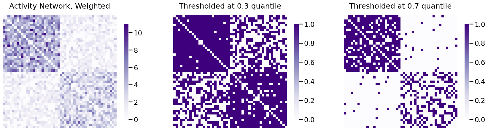
Great job. Next, we will discuss an important property as to why thresholding using a quantile tends to be a very common tactic to obtaining simple networks from networks which are undirected and loopless. Remember that in the The network density indicates the fraction of possible edges which exist, we defined the network density for a simple network as:

\[\begin{align*} density(A) &= \frac{2\sum_{j > i}a_{ij}}{n(n - 1)}. \end{align*}\]

Since you have thresholded at the \(0.3\) quantile for the activity network, this means that about \(70\) percent of the possible edges will exist (the largest \(70\) percent of edges), and \(30\) percent of the possible edges will not exist (the smallest \(30\) percent of edges). Remembering that the number of possible edges was \(\frac{1}{2}n(n - 1)\) for an undirected network, this means that \(\sum_{j > i}a_{ij}\) must be \(0.7\) of \(\frac{1}{2}n(n - 1)\), or \(\frac{7}{20}n(n - 1)\). Therefore:

\[\begin{align*} density(A) &= \frac{2\sum_{j > i}a_{ij}}{n(n - 1)}, \\ &= \frac{2\cdot \frac{7}{20}n(n - 1)}{n(n - 1)},\;\;\;\sum_{j > i}a_{ij} = \frac{7}{20}n(n - 1) \\ &= 0.7. \end{align*}\]

So when you threshold the network at a quantile \(q\), you end with a network of density equal to \(1 - q\)! Let’s confirm that this is the case for your activity network thresholded at \(0.3\):

from graspologic.utils import is_unweighted, is_loopless, is_symmetric

def simple_network_dens(X):
    # make sure the network is simple
    if (not is_unweighted(X)) or (not is_loopless(X)) or (not is_symmetric(X)):
        raise TypeError("Network is not simple!")
    # count the non-zero entries in the upper-right triangle
    # for a simple network X
    nnz = np.triu(X, k=1).sum()
    # number of nodes
    n = X.shape[0]
    # number of possible edges is 1/2 * n * (n-1)
    poss_edges = 0.5*n*(n-1)
    return nnz/poss_edges

print("Network Density: {:.3f}".format(simple_network_dens(A_activity_thresholded03)))

Network Density: 0.700

This is desirable for network machine learning because many network properties (such as the summary statistics we have discussed so far, and numerous other properties we will discuss in later chapters) can vary when the network density changes. This means that a network of a different density might have a higher clustering coefficient than a network of a lower density simply due to the fact that its density is higher (and therefore, there are more opportunities for closed triangles because each node has more connections). This means that when you threshold groups of networks and compare them, thresholding using a quantile will be very valuable.

3.4.2.3.1.3. Remember to be careful with quantiles!#

Note that a common pitfall you might run into with sparsification approaches that rely on quantiles occurs when a weighted network can only take non-negative edge-weights. This corresponds to a network with an adjacency matrix \(A\) where every \(a_{ij}\) is greater than or equal to \(0\). In this case, one must be careful about the implementation of sparsification. Imagine, for instance, that you have a network in which \(50\%\) of the possible edges do not exist and have an adjacency entry of \(0\), and \(50\%\) of the possible edges exist and have an adjacency entry of \(1\) (the network density is \(0.5\)). If you threshold this network at the \(0.3\) quantile, you will have a cutoff of \(0\), and if you don’t handle ties appropriately, the network will remain identical before and after thresholding. This means that while you would expect the network density to be \(1 - 0.3 = 0.7\), you would still have a network with a density of \(0.5\). This is why we went to such great lengths to appropriately handle ties in the quantile function: so that we could preserve the desired network density. When do you think you wouldn’t have to worry about this when truncating or thresholding?

A network needs to satisfy two properties for you to not have to worry about ties. First, if it is weighted, the network needs to take continuous real values: this means that the edge-weights need to take arbitrary values in a particular interval, and not be biased towards any particular fixed values. If the edge-weights take continuous values, that means that the probability of any two edge-weights being identical is exactly zero, so ties will not be possible! Further, the network must be dense. A network is dense if all possible edges exist, with possibly arbitrarily low or high edge-weights. When the network is dense, this means that the

3.4.2.3.2. Edge-weight global rescaling#

With weighted networks, it is often the case that you might want to reshape the distributions of edge-weights in your networks to highlight particular properties. Notice that the edge-weights for your friendship network takes values between \(0\) and \(1\), but your activity network takes values between \(0\) and almost \(15\). How can you possibly compare between these two networks where the edge-weights take such different ranges of values? You turn to standardization, which allows us to place values from different networks on the same scale.

3.4.2.3.2.1. \(z\)-scoring standardizes edge weights using the normal distribution#

The first approach to edge-weight standardization is known commonly as \(z\)-scoring. Suppose that \(A\) is the adjacency matrix, with entries \(a_{ij}\). With a \(z\)-score, you will rescale the weights of the adjacency matrix, such that the new edge-weights (called \(z\)-scores) are approximately normally distributed. The reason this can be useful is that the normal distribution is pretty ubiquitous across many branches of science, and therefore, a \(z\)-score is relatively easy to communicate with other scientists. Further, many things that exist in nature can be well-approximated by a normal distribution, so it seems like a reasonable place to start to use a \(z\)-score for edge-weights, too! The \(z\)-score is defined as follows. You will construct the \(z\)-scored adjacency matrix \(Z\), whose entries \(z_{ij}\) are the corresponding \(z\)-scores of the adjacency matrix’s entries \(a_{ij}\). For a weighted, loopless network, you use an estimate of the mean, \(\hat \mu\), and the unbiased estimate of the variance, \(\hat \sigma^2\)), which can be computed as follows:

\[\begin{align*} \hat\mu &= \frac{1}{n}\sum_{i \neq j}a_{ij},\\ \hat\sigma^2 &= \frac{1}{n - 1}\sum_{i \neq j} (a_{ij} - \hat\mu)^2. \end{align*}\]

The \(z\)-score for the \((i,j)\) entry is simply the quantity:

\[\begin{align*} z_{ij} &= \frac{a_{ij} - \hat\mu}{\hat\sigma} \end{align*}\]

Since your network is loopless, notice that these sums are for all non-diagonal entries where \(i \neq j\). If the network were not loopless, you would include diagonal entries in the calculation, and instead would sum over all possible combinations of \(i\) and \(j\). the interpretation of the \(z\)-score \(z_{ij}\) is the number of stadard deviations that the entry \(a_{ij}\) is from the mean, \(\hat \mu\).

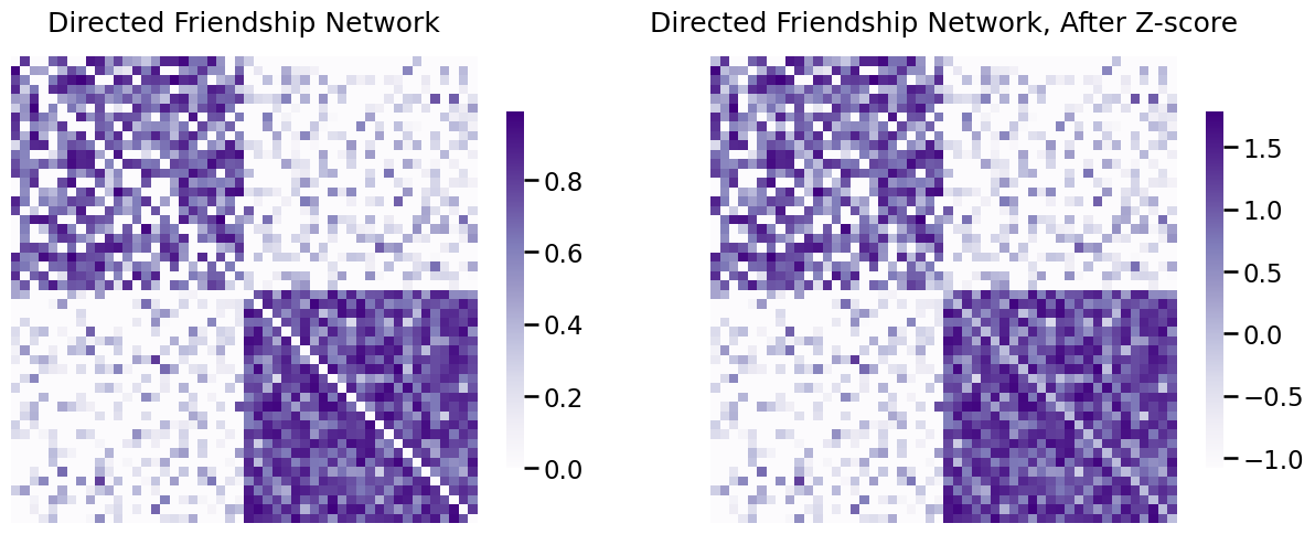
We will demonstrate on the directed friendship network. You can implement \(z\)-scoring as follows:

from scipy.stats import zscore

def z_score_loopless(X):
    if not is_loopless(X):
        raise TypeError("The network has loops!")
    # the entries of the adjacency matrix that are not on the diagonal
    non_diag_idx = np.where(~np.eye(X.shape[0], dtype=bool))
    Z = np.zeros(X.shape)
    Z[non_diag_idx] = zscore(X[non_diag_idx])
    return Z

ZA_friend = z_score_loopless(A_friend)

fig, axs = plt.subplots(1,2, figsize=(15, 6))

heatmap(A_friend, ax=axs[0], title="Directed Friendship Network")
heatmap(ZA_friend, ax=axs[1], title="Directed Friendship Network, After Z-score");

Next, you will look at the edge-weight histogram for the directed friendship network before and after \(z\)-scoring. Remember that the network is loopless, so again you exclude the diagonal entries:

from seaborn import histplot

non_diag_idx = np.where(~np.eye(A_friend.shape[0], dtype=bool))
fig, axs = plt.subplots(1,2, figsize=(15, 4))
ax = histplot(A_friend[non_diag_idx].flatten(), ax=axs[0], bins=9)
ax.set_xlabel("Edge Weight");
ax.set_ylabel("Number of Edges");
ax.set_title("Directed Friendship Network, Before Z-score");
ax = histplot(ZA_friend[non_diag_idx].flatten(), ax=axs[1], bins=9)
ax.set_xlabel("Z-score");
ax.set_ylabel("Number of Edges");
ax.set_title("Directed Friendship Network, After Z-score");

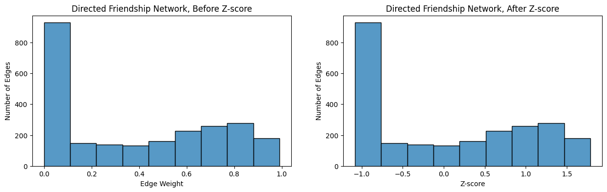
The theory for when, and why, to use \(z\)-scoring for network machine learning tends to go something like this: many things tend to be normally distributed with the same mean and variance, so perhaps that is a reasonable expectation for your network, too. Unfortunately, we find this often to not be the case. In fact, we often find that the specific distribution of edge weights itself often might be lamost infeasible to identify in a population of networks, and therefore almost irrelevant all-together. To this end, we turn to instead ranking the edges.

3.4.2.3.2.2. Ranking edges preserves ordinal relationships#

The idea behind ranking is as follows. You don’t really know much useful information as to how the distribution of edge weights varies between a given pair of networks. For this reason, you want to virtually eliminate the impact of that distribution almost entirely. However, you know that if one edge-weight is larger than another edge-weight, that you do in fact trust that relationship. What this means is that you want something which preserves ordinal relationships in your edge-weights, but ignores other properties of the edge-weights. An ordinal relationship just means that you have a natural ordering to the edge-weights. This means that you can identify a largest edge-weight, a smallest edge-weight, and every position in between. When you want to preserve ordinal relationships in your network, you do something called passing the non-zero edge-weights to ranks. We will often use the abbreviation ptr to define this function because it is so useful for weighted networks. You pass non-zero edge-weights to ranks as follows:

Identify all of the non-zero entries of the adjacency matrix \(A\).
Count the number of non-zero entries of the adjacency matrix \(A\), \(n_{nz}\).
Rank all of the non-zero edges in the adjacency matrix \(A\), where for a non-zero entry \(a_{ij}\), \(rank(a_{ij}) = 1\) if \(a_{ij}\) is the smallest non-zero edge-weight, and \(rank(a_{ij}) = n_{nz}\) if \(a_{ij}\) is the largest edge-weight. Ties are settled by using the average rank of the two entries.
Report the weight of each non-zero entry \((i,j)\) as \(r_{ij} = \frac{rank(a_{ij})}{n_{nz} + 1}\), and for eachh zero entry as \(r_{ij} = 0\).

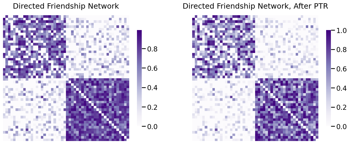
Below, you pass-to-ranks the directed friendship network using graspologic, showing both the adjacency matrix and the edge-weight distribution before and after ptr:

from graspologic.utils import pass_to_ranks

RA_friend = pass_to_ranks(A_friend)

fig, axs = plt.subplots(1,2, figsize=(15, 6))

heatmap(A_friend, ax=axs[0], title="Directed Friendship Network")
heatmap(RA_friend, ax=axs[1], title="Directed Friendship Network, After PTR", vmin=0, vmax=1);

fig, axs = plt.subplots(1,2, figsize=(15, 4))
ax = histplot(A_friend[non_diag_idx].flatten(), ax=axs[0], bins=9)
ax.set_xlabel("Edge Weight");
ax.set_ylabel("Number of Edges");
ax.set_title("Directed Friendship Network, Before PTR");
ax = histplot(RA_friend[non_diag_idx].flatten(), ax=axs[1], binrange=[0, 1], bins=9)
ax.set_xlabel("normalized rank");
ax.set_ylabel("Number of Edges");
ax.set_title("Directed Friendship Network, After PTR");

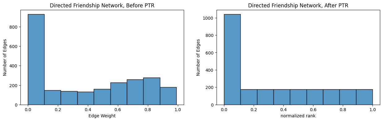
The edge-weights for the adjacency matrix \(R\) after ptr has the interpretation that each entry \(r_{ij}\) which is non-zero is the quantile of that entry amongst the other non-zero entries. This is unique in that it is completely distribution-free, which means that you don’t need to assume anything about the distribution of the edge-weights to have an interpretable quantity. On the other hand, the \(z\)-score had the interpretation of the number of standard deviations from the mean, which is only a sensible quantity to compare if you assume the population of edge-weights are normally distributed.

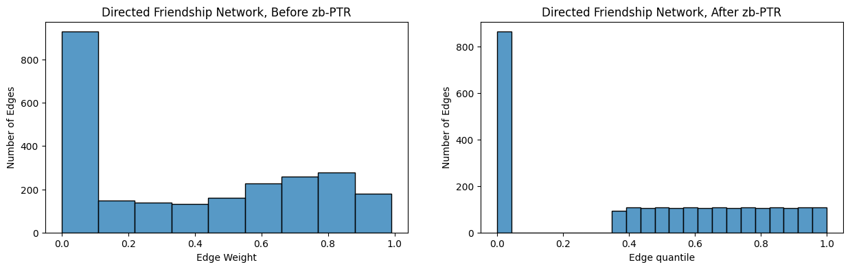
Another useful quantity related to pass-to-ranks is known as the zero-boosted pass-to-ranks. Zero-boosted pass-to-ranks is conducted as follows:

Identify all of the non-zero entries of the adjacency matrix \(A\).
Count the number of non-zero entries of the adjacency matrix \(A\), \(n_{nz}\), and the number of zero-entries of the adjacency matrix \(A\), \(n_z\). Note that since the values of the adjacency matrix are either zero or non-zero, that \(n_{nz} + n_z = n^2\), as \(A\) is an \(n \times n\) matrix and therefore has \(n^2\) total entries.
Rank all of the non-zero edges in the adjacency matrix \(A\), where for a non-zero entry \(a_{ij}\), \(rank(a_{ij}) = 1\) if \(a_{ij}\) is the smallest non-zero edge-weight, and \(rank(a_{ij}) = n_{nz}\) if \(a_{ij}\) is the largest edge-weight. Ties are settled by using the average rank of the two entries.
Report the weight of each non-zero entry \((i,j)\) as \(r_{ij}' = \frac{n_z + rank(a_{ij})}{n^2 + 1}\), and for each zero entry as \(r_{ij}' = 0\).

The edge-weights for the adjacency matrix \(R'\) after zero-boosted ptr have the interpretation that each entry \(r_{ij}'\) is the quantile of that entry amongst all of the entries. Let’s instead use zero-boosted ptr on your network:

RA_friend_zb = pass_to_ranks(A_friend, method="zero-boost")

fig, axs = plt.subplots(1,2, figsize=(15, 4))
ax = histplot(A_friend[non_diag_idx].flatten(), ax=axs[0], bins=9)
ax.set_xlabel("Edge Weight");
ax.set_ylabel("Number of Edges");
ax.set_title("Directed Friendship Network, Before zb-PTR");
ax = histplot(RA_friend_zb[non_diag_idx].flatten(), ax=axs[1], binrange=[0, 1], bins=23)
ax.set_xlabel("Edge quantile");
ax.set_ylabel("Number of Edges");
ax.set_title("Directed Friendship Network, After zb-PTR");

As it turns out, the thresholding approach you learned above can be thought of as a decimation of ranking, assuming that the ranking implementation handles ties randomly (the implementation in graspologic does not, as ties are settled by the average rank, but we would encourage you to implement one that does as an exercise). For instance, if you picked a threshold of \(0.5\), there is some corresponding rank (or value in between two ranks), where all of the elements of the adjacency matrix with a rank lower than a given threshold \(\tau_r\) have corresponding weights lower than \(\tau\) and all of the elements of the adjacency matrix with a rank higher than a given threshold \(\tau_r\) have corresponding weights higher than \(\tau\). Then, you can simply threshold the ranked adjacency matrix using \(\tau_r\).

3.4.2.3.2.3. Logging reduces magnitudinal differences between edges#

When you look at the distribution of non-zero edge-weights for the activity/hobby network or the friendship network, you notice a strange pattern, known as a right-skew:

fig, ax = plt.subplots(1,1, figsize=(15, 5))
ax = histplot(A_activity.flatten(), ax=ax, bins=10)
ax.set_xlabel("Edge Weight");
ax.set_ylabel("Number of Edges");
ax.set_title("Activity/Hobby Network Edge Distribution");

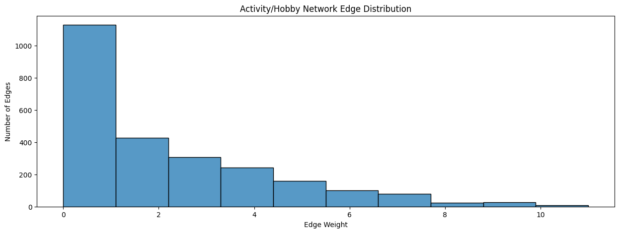
Notice that most of the edges have weights which are comparatively small, between \(0\) and \(34\), but some of the edges have weights which are much (much) larger. A right-skew exists when the majority of edge-weights are small, but some of the edge-weights take values which are much larger.

What if you want to make these large values more similar in relation to the smaller values, but you simultaneously want to preserve properties of the underlying distribution of the edge-weights? Well, you can’t use ptr, because ptr will throw away all of the information about the edge-weight distribution other than the ordinal relationship between pairs of edges. To interpret what this means, you might think that there is a big difference between sharing no interests compared to three interests in common, but there is not as much of a difference in sharing ten interests compared to thirteen interests in common.

To do this, you instead turn to the logarithm function. The logarithm function \(log_{10}(x)\) is defined for positive values \(x\) as the value \(c_x\) where \(x = 10^{c_x}\). In this sense, it is the “number of powers of ten” to obtain the value \(x\). You will notice that the logarithm function looks like this:

import warnings
warnings.filterwarnings('ignore')
import seaborn as sns

xs = np.linspace(0.001, 100, num=1000)
logxs = np.log10(xs)

fig, ax = plt.subplots(1,1, figsize=(8, 6))
sns.lineplot(xs, logxs, ax=ax)
ax.axhline(0, color="red")
ax.set_xlabel("x")
ax.set_ylabel("$log_{10}(x)$");

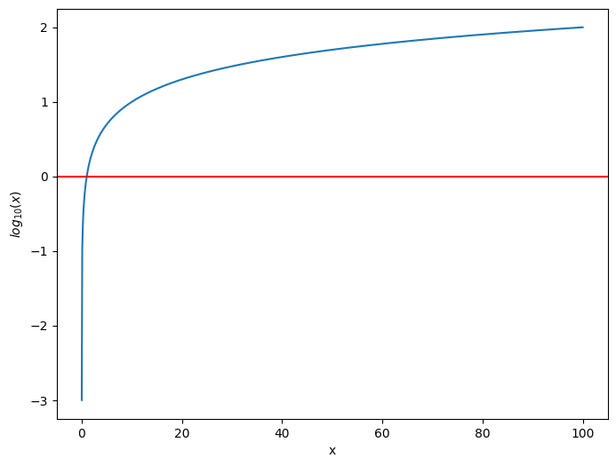
What is key to noice about this function is that, as \(x\) increases, the log of \(x\) increases by a decreasing amount. Let’s imagine you have three values, \(x = .001\), \(y = .1\), and \(z = 10\). A calculator will give you that \(log_{10}(x) = -3, log_{10}(y) = -1\), and \(log_{10}(z) = 1\). Even though \(y\) is only \(.099\) units bigger than \(x\), its logarithm \(log_{10}(y)\) exceeds \(log_{10}(x)\) by two units. on the other hand, \(z\) is \(9.9\) units bigger than \(y\), but yet its logarithm \(log_{10}(z)\) is still the same two units bigger than \(log_{10}(y)\). This is because thhe logarithm is instead looking at the fact that \(z\) is one power of ten, \(y\) is \(-1\) powers of ten, and \(z\) is \(-3\) powers of ten. The logarithm has collapsed the huge size difference between \(z\) and the other two values \(x\) and \(y\) by using exponentiation with base ten.

In this sense, you can also use the logarithm function for your network to reduce the huge size difference between the values in your activity/hobby network. However, we must first add a slight twist: to do this properly and yield an interpretable adjacency matrix, you need to augment the entries of the adjacency matrix if it contains zeros. This is because the \(log_{10}(0)\) is not defined. To augment the adjacency matrix, you will use the following strategy:

Identify the entries of \(A\) which take a value of zero.
Identify the smallest entry of \(A\) which is not-zero, and call it \(a_m\).
Compute a value \(\epsilon\) which is an order of magnitude smaller than \(a_m\). Since you are taking powers of ten, a single order of magnitude would give us that \(\epsilon = \frac{a_m}{10}\).
Take the augmented adjacency matrix \(A'\) to be defined with entries \(a_{ij}' = a_{ij} + \epsilon\).

Next, since your matrix has values which are now all greater than zero, you can just take the logarithm:

def augment_zeros(X):
    if np.any(X < 0):
        raise TypeError("The logarithm is not defined for negative values!")
    am = np.min(X[np.where(X > 0)])  # the smallest non-zero entry of X
    eps = am/10  # epsilon is one order of magnitude smaller than the smallest non-zero entry
    return X + eps  # augment all entries of X by epsilon

A_activity_aug = augment_zeros(A_activity)
# log-transform using base 10
A_activity_log = np.log10(A_activity_aug)

fig, axs = plt.subplots(1,2, figsize=(15, 6))

heatmap(A_activity, ax=axs[0], title="Activity/Hobby Network Network")
heatmap(A_activity_log, ax=axs[1], title="Activity/Hobby Network, After Augmentation + log");

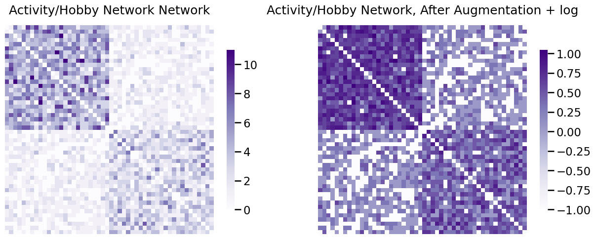
When you plot the augmented and log-transformed data, what you see is that many of the edge-weights you originally might have thought were zero if you only looked at a plot were, in actuality, not zero. In this sense, for non-negative weighted networks, log transforming after zero-augmentation is often very useful for visualization to get a sense of the magnitudinal differences that might be present between edges.

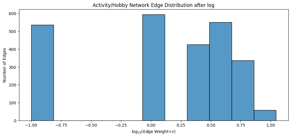
Our edge-weight histogram becomes:

fig, ax = plt.subplots(1,1, figsize=(12, 5))
ax = histplot(A_activity_log.flatten(), ax=ax, bins=11)
ax.set_xlabel("$log_{10}($Edge Weight$ + \epsilon)$");
ax.set_ylabel("Number of Edges");
ax.set_title("Activity/Hobby Network Edge Distribution after log");

3.4.3. References#

1: Albert-Lszl Barabsi. Network science. Philos. Trans. Royal Soc. A, 371(1987):20120375, March 2013. doi:10.1098/rsta.2012.0375.
2: Trevor Hastie, Robert Tibshirani, and Jerome H. Friedman. The Elements of Statistical Learning: Data Mining, Inference, and Prediction. Springer, New York, NY, USA, 2009. ISBN 978-0-38784884-6. URL: https://books.google.com/books/about/The_Elements_of_Statistical_Learning.html?id=eBSgoAEACAAJ&source=kp_book_description.
3: Daniel A. Spielman and Shang-Hua Teng. Spectral Sparsification of Graphs. arXiv, August 2008. arXiv:0808.4134, doi:10.48550/arXiv.0808.4134.
4: Joshua Batson, Daniel A. Spielman, Nikhil Srivastava, and Shang-Hua Teng. Spectral sparsification of graphs: theory and algorithms. Commun. ACM, 56(8):87–94, August 2013. doi:10.1145/2492007.2492029.

Hands-on Network Machine Learning with Scikit-Learn and Graspologic

Regularization

Contents