2.4. Select and Train a Model

So, now you’ve got your data loaded and pre-processed… what next? Let’s get all the code in that we’ve used so far:

import warnings
warnings.filterwarnings("ignore")

import os
import urllib
import boto3
from botocore import UNSIGNED
from botocore.client import Config
from graspologic.utils import import_edgelist, pass_to_ranks
import numpy as np
from sklearn.base import TransformerMixin, BaseEstimator
from sklearn.pipeline import Pipeline
import glob

# the AWS bucket the data is stored in
BUCKET_ROOT = "open-neurodata"
parcellation = "Schaefer400"
FMRI_PREFIX = "m2g/Functional/BNU1-11-12-20-m2g-func/Connectomes/" + parcellation + "_space-MNI152NLin6_res-2x2x2.nii.gz/"
FMRI_PATH = os.path.join("datasets", "fmri")  # the output folder
DS_KEY = "abs_edgelist"  # correlation matrices for the networks to exclude

def fetch_fmri_data(bucket=BUCKET_ROOT, fmri_prefix=FMRI_PREFIX,
                    output=FMRI_PATH, name=DS_KEY):
    """
    A function to fetch fMRI connectomes from AWS S3.
    """
    # check that output directory exists
    if not os.path.isdir(FMRI_PATH):
        os.makedirs(FMRI_PATH)
    # start boto3 session anonymously
    s3 = boto3.client('s3', config=Config(signature_version=UNSIGNED))
    # obtain the filenames
    bucket_conts = s3.list_objects(Bucket=bucket, 
                    Prefix=fmri_prefix)["Contents"]
    for s3_key in bucket_conts:
        # get the filename
        s3_object = s3_key['Key']
        # verify that we are grabbing the right file
        if name not in s3_object:
            op_fname = os.path.join(FMRI_PATH, str(s3_object.split('/')[-1]))
            if not os.path.exists(op_fname):
                s3.download_file(bucket, s3_object, op_fname)

def read_fmri_data(path=FMRI_PATH):
    """
    A function which loads the connectomes as adjacency matrices.
    """
    # import edgelists with graspologic
    # edgelists will be all of the files that end in a csv
    networks = [import_edgelist(fname) for fname in glob.glob(os.path.join(path, "*.csv"))]
    return networks

def remove_isolates(A):
    """
    A function which removes isolated nodes from the 
    adjacency matrix A.
    """
    degree = A.sum(axis=0)  # sum along the rows to obtain the node degree
    out_degree = A.sum(axis=1)
    A_purged = A[~(degree == 0),:]
    A_purged = A_purged[:,~(degree == 0)]
    print("Purging {:d} nodes...".format((degree == 0).sum()))
    return A_purged

class CleanData(BaseEstimator, TransformerMixin):
    def __init__(self):
        return
    def fit(self, X):
        return self

    def transform(self, X):
        print("Cleaning data...")
        Acleaned = remove_isolates(X)
        A_abs_cl = np.abs(Acleaned)
        self.A_ = A_abs_cl
        return self.A_
    
class FeatureScaler(BaseEstimator, TransformerMixin):
    def __init__(self):
        return
    
    def fit(self, X):
        return self
    
    def transform(self, X):
        print("Scaling edge-weights...")
        A_scaled = pass_to_ranks(X)
        return (A_scaled)

num_pipeline = Pipeline([
    ('cleaner', CleanData()),
    ('scaler', FeatureScaler()),
])

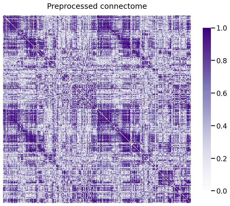
from graphbook_code import heatmap

fetch_fmri_data()
As = read_fmri_data()
A = As[0]

A_xfm = num_pipeline.fit_transform(A)
heatmap(A_xfm, title="Preprocessed connectome", vmin=0, vmax=1);

Cleaning data...
Purging 0 nodes...
Scaling edge-weights...

2.4.1. Generating new representations from your data

As you were briefly introduced to in Section 1.1 and will cover more thoroughly in Section 5, a major problem with learning from network data is that, inherently, networks in their rawest form are not tabular datasets. This means that if you want to apply any of the breadth of knowledge that has been acquired in general machine learning (which is typically designed for tabular datasets), you need to learn how to adapt your network to be compatible with tabular approaches, or learn how to adapt your general machine learning architecture for network layouts, such as adjacency matrices, which properly convey the dependences in network data.

As you will learn, particularly in the end of this book in Section 9, the former is possible, but generally a bit more involved. The latter approach tends to be, in our opinions, a bit more straightforward at first, and is usually fantastic for most applications. So, how do you obtain a tabular representation of your dataset?

Well, one possible thing you can do is you can use something called a Section 5.3, a technique that you will learn has a wide range of applications in network machine learning whether you are studying one network, pairs of networks, or multiple networks. Let’s see what happens when we spectrally embed our connectome:

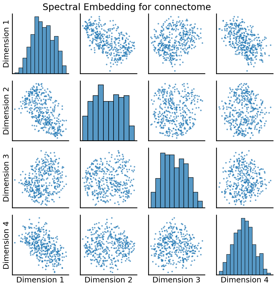
from graspologic.embed import AdjacencySpectralEmbed

embedding = AdjacencySpectralEmbed().fit_transform(A_xfm)

An embedding takes the adjacency matrix, which is a matrix representation of the entire network, and turns it into a tabular array. Each row is called an estimated latent position for a given node, and each column is called an estimated latent dimension of the network. This means that if there are \(n\) nodes, there are \(n\) rows of the spectral embedding, and if there are \(d\) estimated latent dimensions of the network, there are \(d\) columns. Overall, the spectral embedding has taken the \(n \times n\) adjacency matrix, which we can’t inherently use network machine learning algorithms on, and transformed it into a \(n \times d\) tabular array, which we can inherently use machine learning algorithms on. We’ll visualize this embedding using a pairs plot, which as you will learn later, is a scatter plot showing where each node is a single point in the plot, and the x and y axes are different pairs of latent dimensions for that particular node:

from graspologic.plot import pairplot

_ = pairplot(embedding, title="Spectral Embedding for connectome")

As it turns out, this particular representation of the adjacency matrix through the spectral embedding can, optionally, be tied into a statistical model if you make some assumptions; particularly, those of the stochastic block model, which you will learn about in chapter 5. Basically, what the stochastic block model says is that each node is a member of a subgroup, called a community, and its connectivity to other nodes in the network is dictated by which community it is a member of, and which community the other node is a member of. This sounds a lot like the question that your colleague wanted you to approach, since he wanted a way to take the nodes of the network and form “functionally similar” subgroups from them.

Now that we have a tabular representation of the data, we can take attempt to use the intuition and assumptions of the stochastic block model to cluster our nodes. Let’s see what happens when we apply \(k\)-means to our data:

from sklearn.cluster import KMeans

labels = KMeans(n_clusters=2).fit_predict(embedding)

_ = pairplot(embedding, labels=labels, legend_name="Predicter Clusters", title="KMeans clustering")

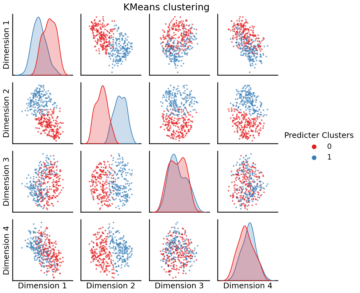
So, it looks like the \(k\)-means was able to learn \(2\) clusters from our dataset. These clusters are indicated by the “blobs” of points that are red or blue, respectively.

If you’re careful, you’ll notice we did something a little weird here. Why did we choose \(2\)? Why not \(5\)? Why not \(8\)? We chose \(2\) here somewhat arbitrarily. In general, when you don’t know what to expect from your data (we didn’t know what to expect here, other than that we wanted a modestly sized way to group the nodes up), it’s a good idea to use quantitative means to make these determinations for you.

With KMeans(), we can use something called the silhouette score to do this for us. You choose the optimal number of clusters as the clustering with the highest silhouette score. You’ll learn a lot more about the silhouette score when you learn about community detection. graspologic makes this process pretty straightforward:

from graspologic.cluster import KMeansCluster

labels = KMeansCluster(max_clusters=10).fit_predict(embedding)

_ = pairplot(embedding, labels=labels, title="KMeans clustering, automatic selection", legend_name="Predicted Clusters")

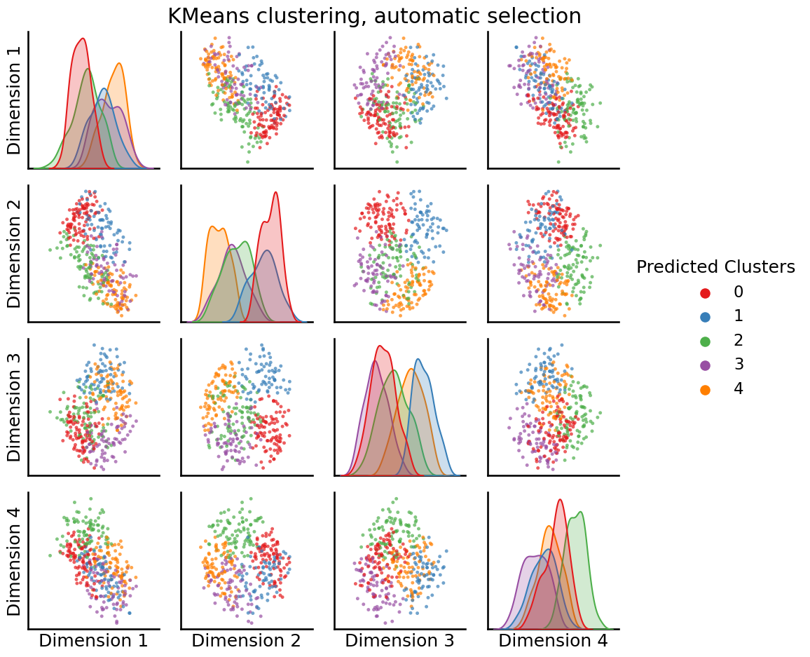
Unlike the previous approach, it looks like with silhouette score selection, we ended up with \(3\) clusters being optimal, not \(2\).

So, what about other possible approaches? Unless you are pretty confident that the clusters you are looking for have “blobs” that are totally spherically symmetric (basically, they look like “balls” in the dataset), \(k\)-means can be a pretty bad idea. As you’ll learn later, another strategy called the gaussian mixture model, or GMM, handles this a bit more elegantly, and allows your cluster blobs to be pretty much any ellipse-like shape. We can use GMM and automatically select the number of clusters using the Bayesian Information Criterion, or BIC, with AutoGMMCluster:

from graspologic.cluster import AutoGMMCluster

labels = AutoGMMCluster(max_components=10).fit_predict(embedding)

_ = pairplot(embedding, labels=labels, title="AutoGMM Clustering", legend_name="Predicted Clusters")

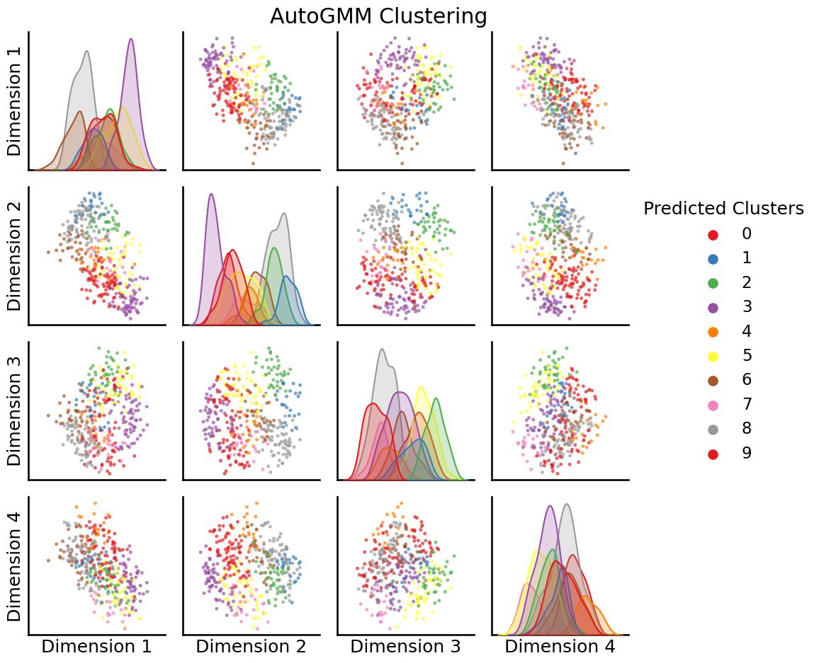
So, it looks like GMM actually found \(4\) clusters to be a bit more optimal than \(3\) clusters.