Plot the projection matrices of an oblique tree for sampling images, or time-series

This example shows how projection matrices are generated for an oblique tree, specifically the treeple.tree.PatchObliqueDecisionTreeClassifier.

For a tree, one can specify the structure of the data that it will be trained on (i.e. (X, y)). This is done by specifying the data_dims parameter. For example, if the data is 2D, then data_dims should be set to (n_rows, n_cols), where now each row of X is a 1D array of length n_rows * n_cols. If the data is 3D, then data_dims should be set to (n_rows, n_cols, n_depth), where now each row of X is a 1D array of length n_rows * n_cols * n_depth. This allows the tree to be trained on data of any structured dimension, but still be compatible with the robust sklearn API.

The projection matrices are used to generate patches of the data. These patches are used to calculate the feature values that are used during splitting. The patch is generated by sampling a hyperrectangle from the data. The hyperrectangle is defined by a starting point and a patch size. The starting point is sampled uniformly from the structure of the data. For example, if each row of X has a 2D image structure (n_rows, n_cols), then the starting point will be sampled uniformly from the square grid. The patch size is sampled uniformly from the range min_patch_dims to max_patch_dims. The patch size is also constrained to be within the bounds of the data structure. For example, if the patch size is (3, 3) and the data structure is (5, 5), then the patch will only sample indices within the data.

We also allow each dimension to be arbitrarily discontiguous.

For details on how to use the hyperparameters related to the patches, see treeple.tree.PatchObliqueDecisionTreeClassifier.

import matplotlib.pyplot as plt

# import modules
# .. note:: We use a private Cython module here to demonstrate what the patches
#           look like. This is not part of the public API. The Cython module used
#           is just a Python wrapper for the underlying Cython code and is not the
#           same as the Cython splitter used in the actual implementation.
#           To use the actual splitter, one should use the public API for the
#           relevant tree/forests class.
import numpy as np

from treeple._lib.sklearn.tree._criterion import Gini
from treeple.tree.manifold._morf_splitter import BestPatchSplitterTester

Initialize patch splitter

The patch splitter is used to generate patches for the projection matrices. We will initialize the patch with some dummy values for the sake of this example.

criterion = Gini(1, np.array((0, 1)))
max_features = 6
min_samples_leaf = 1
min_weight_leaf = 0.0
random_state = np.random.RandomState(100)

boundary = None
feature_weight = None
monotonic_cst = None
missing_value_feature_mask = None

# initialize some dummy data
X = np.repeat(np.arange(25).astype(np.float32), 5).reshape(5, -1)
y = np.array([0, 0, 0, 1, 1]).reshape(-1, 1).astype(np.float64)
sample_weight = np.ones(5)

print("The shape of our dataset is: ", X.shape, y.shape, sample_weight.shape)

The shape of our dataset is:  (5, 25) (5, 1) (5,)

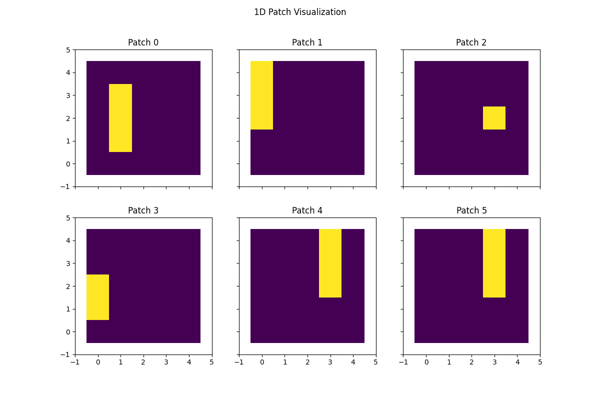
Generate 1D patches

Now that we have th patch splitter initialized, we can generate some patches and visualize how they appear on the data. We will make the patch 1D, which samples multiple rows contiguously. This is a 1D patch of size 3.

Warning

Do not use this interface directly in practice.

min_patch_dims = np.array((1, 1))
max_patch_dims = np.array((3, 1))
dim_contiguous = np.array((True, True))
data_dims = np.array((5, 5))

# Note: not used, but passed for API compatibility
feature_combinations = 1.5

splitter = BestPatchSplitterTester(
    criterion,
    max_features,
    min_samples_leaf,
    min_weight_leaf,
    random_state,
    monotonic_cst,
    feature_combinations,
    min_patch_dims,
    max_patch_dims,
    dim_contiguous,
    data_dims,
    boundary,
    feature_weight,
)
splitter.init_test(X, y, sample_weight, missing_value_feature_mask)

# sample the projection matrix that consists of 1D patches
proj_mat = splitter.sample_projection_matrix_py()
print(proj_mat.shape)

# Visualize 1D patches
fig, axs = plt.subplots(nrows=2, ncols=3, figsize=(12, 8), sharex=True, sharey=True, squeeze=True)
axs = axs.flatten()
for idx, ax in enumerate(axs):
    ax.imshow(proj_mat[idx, :].reshape(data_dims), cmap="viridis")
    ax.set(
        xlim=(-1, data_dims[1]),
        ylim=(-1, data_dims[0]),
        title=f"Patch {idx}",
    )

fig.suptitle("1D Patch Visualization")
plt.show()

(6, 25)

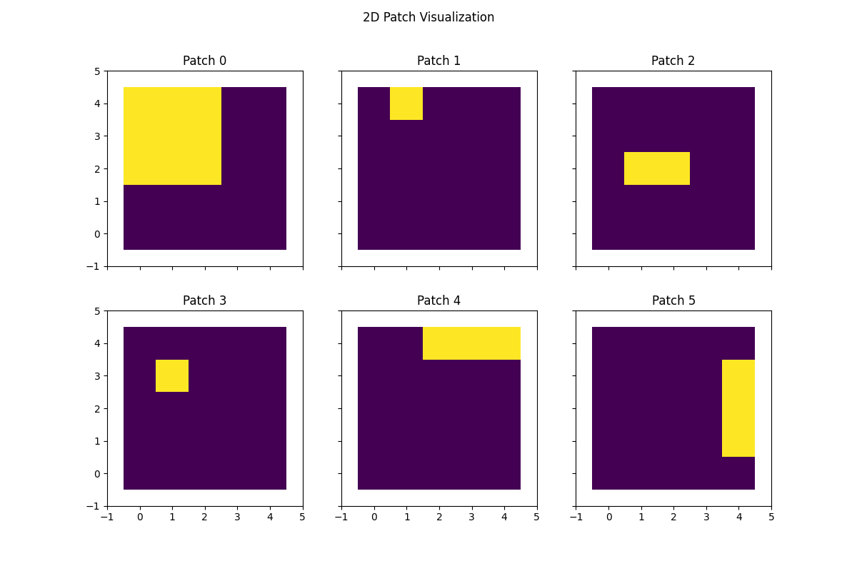
Generate 2D patches

We will make the patch 2D, which samples multiple rows contiguously. This is a 2D patch of size 3 in the columns and 2 in the rows.

min_patch_dims = np.array((1, 1))
max_patch_dims = np.array((3, 3))
dim_contiguous = np.array((True, True))
data_dims = np.array((5, 5))

splitter = BestPatchSplitterTester(
    criterion,
    max_features,
    min_samples_leaf,
    min_weight_leaf,
    random_state,
    monotonic_cst,
    feature_combinations,
    min_patch_dims,
    max_patch_dims,
    dim_contiguous,
    data_dims,
    boundary,
    feature_weight,
)
splitter.init_test(X, y, sample_weight, missing_value_feature_mask)

# sample the projection matrix that consists of 1D patches
proj_mat = splitter.sample_projection_matrix_py()

# Visualize 2D patches
fig, axs = plt.subplots(nrows=2, ncols=3, figsize=(12, 8), sharex=True, sharey=True, squeeze=True)
axs = axs.flatten()
for idx, ax in enumerate(axs):
    ax.imshow(proj_mat[idx, :].reshape(data_dims), cmap="viridis")
    ax.set(
        xlim=(-1, data_dims[1]),
        ylim=(-1, data_dims[0]),
        title=f"Patch {idx}",
    )

fig.suptitle("2D Patch Visualization")
plt.show()

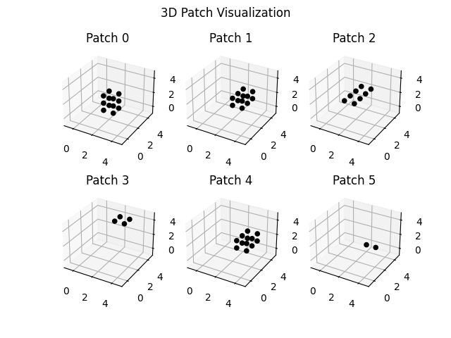
Generate 3D patches

# initialize some dummy data
X = np.repeat(np.arange(25 * 5).astype(np.float32), 5).reshape(5, -1)
y = np.array([0, 0, 0, 1, 1]).reshape(-1, 1).astype(np.float64)
sample_weight = np.ones(5)

# We will make the patch 3D, which samples multiple rows contiguously. This is
# a 3D patch of size 3 in the columns and 2 in the rows.
min_patch_dims = np.array((1, 2, 1))
max_patch_dims = np.array((3, 2, 4))
dim_contiguous = np.array((True, True, True))
data_dims = np.array((5, 5, 5))

splitter = BestPatchSplitterTester(
    criterion,
    max_features,
    min_samples_leaf,
    min_weight_leaf,
    random_state,
    monotonic_cst,
    feature_combinations,
    min_patch_dims,
    max_patch_dims,
    dim_contiguous,
    data_dims,
    boundary,
    feature_weight,
)
splitter.init_test(X, y, sample_weight, missing_value_feature_mask)

# sample the projection matrix that consists of 1D patches
proj_mat = splitter.sample_projection_matrix_py()
print(proj_mat.shape)

fig = plt.figure()
for idx in range(3 * 2):
    ax = fig.add_subplot(2, 3, idx + 1, projection="3d")

    # Plot the surface.
    z, x, y = proj_mat[idx, :].reshape(data_dims).nonzero()
    ax.scatter(x, y, z, alpha=1, marker="o", color="black")

    # Customize the z axis.
    ax.set_zlim(-1.01, data_dims[2])
    ax.set(
        xlim=(-1, data_dims[1]),
        ylim=(-1, data_dims[0]),
        title=f"Patch {idx}",
    )

fig.suptitle("3D Patch Visualization")
plt.show()

(6, 125)

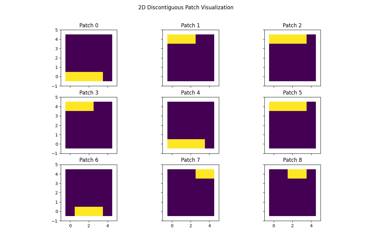
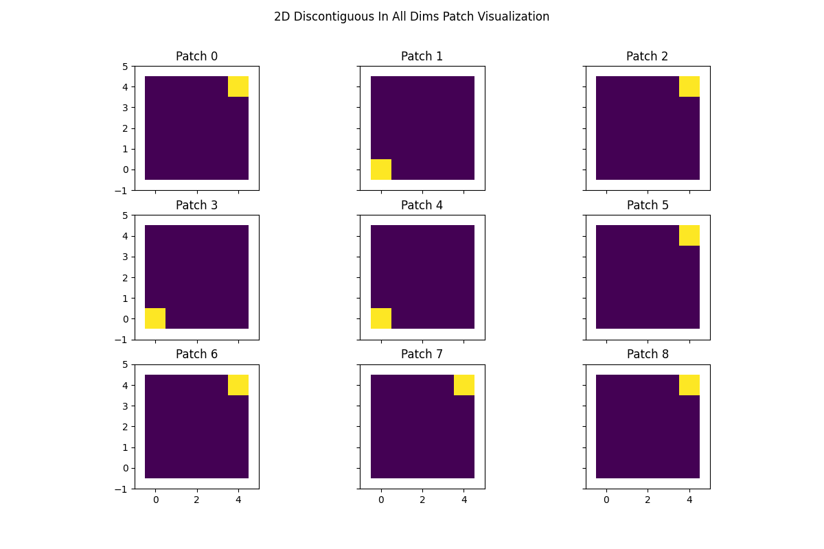
Discontiguous Patches

We can also generate patches that are not contiguous. This is useful for analyzing data that is structured, but not necessarily contiguous in certain dimensions. For example, we can generate patches that sample the data in a multivariate time series, where the data consists of (n_channels, n_times) and the patches are discontiguous in the channel dimension, but contiguous in the time dimension. Here, we show an example patch.

# initialize some dummy data
X = np.repeat(np.arange(25).astype(np.float32), 5).reshape(5, -1)
y = np.array([0, 0, 0, 1, 1]).reshape(-1, 1).astype(np.float64)
sample_weight = np.ones(5)
max_features = 9

# We will make the patch 2D, which samples multiple rows contiguously. This is
# a 2D patch of size 3 in the columns and 2 in the rows.
min_patch_dims = np.array((2, 2))
max_patch_dims = np.array((3, 4))
dim_contiguous = np.array((False, True))
data_dims = np.array((5, 5))

splitter = BestPatchSplitterTester(
    criterion,
    max_features,
    min_samples_leaf,
    min_weight_leaf,
    random_state,
    monotonic_cst,
    feature_combinations,
    min_patch_dims,
    max_patch_dims,
    dim_contiguous,
    data_dims,
    boundary,
    feature_weight,
)
splitter.init_test(X, y, sample_weight, missing_value_feature_mask)

# sample the projection matrix that consists of 1D patches
proj_mat = splitter.sample_projection_matrix_py()

# Visualize 2D patches
fig, axs = plt.subplots(nrows=3, ncols=3, figsize=(12, 8), sharex=True, sharey=True, squeeze=True)
axs = axs.flatten()
for idx, ax in enumerate(axs):
    ax.imshow(proj_mat[idx, :].reshape(data_dims), cmap="viridis")
    ax.set(
        xlim=(-1, data_dims[1]),
        ylim=(-1, data_dims[0]),
        title=f"Patch {idx}",
    )

fig.suptitle("2D Discontiguous Patch Visualization")
plt.show()

We will make the patch 2D, which samples multiple rows contiguously. This is a 2D patch of size 3 in the columns and 2 in the rows.

dim_contiguous = np.array((False, False))

splitter = BestPatchSplitterTester(
    criterion,
    max_features,
    min_samples_leaf,
    min_weight_leaf,
    random_state,
    monotonic_cst,
    feature_combinations,
    min_patch_dims,
    max_patch_dims,
    dim_contiguous,
    data_dims,
    boundary,
    feature_weight,
)
splitter.init_test(X, y, sample_weight, missing_value_feature_mask)

# sample the projection matrix that consists of 1D patches
proj_mat = splitter.sample_projection_matrix_py()

# Visualize 2D patches
fig, axs = plt.subplots(nrows=3, ncols=3, figsize=(12, 8), sharex=True, sharey=True, squeeze=True)
axs = axs.flatten()
for idx, ax in enumerate(axs):
    ax.imshow(proj_mat[idx, :].reshape(data_dims), cmap="viridis")
    ax.set(
        xlim=(-1, data_dims[1]),
        ylim=(-1, data_dims[0]),
        title=f"Patch {idx}",
    )

fig.suptitle("2D Discontiguous In All Dims Patch Visualization")
plt.show()

Estimated memory usage: 228 MB