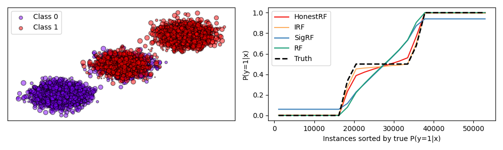
Plot honest forest calibrations on overlapping gaussian simulations

Compare the prediction results of honest forests and random forests with various methods of calibrations. Honest trees are a method for achieving improved calibration in random forests. See User Guide for more information.

Other methods for achieving calibrated random forests are also included:

• Isotonic regression (IRF)

• Sigmoid calibration (SigRF)

• regular Random Forests without calibration (RF)

The plot shows the calibration curves of the different methods on a simulated dataset with two overlapping gaussian clusters. The red line shows the calibration curve of the honest forest, which is closest to the ideal. The figure is reproduced from [1].

References

[1]

Ronan Perry, Ronak Mehta, Richard Guo, Eva Yezerets, Jesús Arroyo, Mike Powell, Hayden Helm, Cencheng Shen, and Joshua T. Vogelstein. Random forests for adaptive nearest neighbor estimation of information-theoretic quantities. arXiv, 2021. arXiv:1907.00325.

Import the necessary modules and libraries

import matplotlib.pyplot as plt
import numpy as np
from matplotlib import cm
from sklearn import datasets
from sklearn.calibration import CalibratedClassifierCV
from sklearn.ensemble import RandomForestClassifier
from sklearn.model_selection import train_test_split

from treeple.ensemble import HonestForestClassifier

Define the classifiers and generate the data

color_dict = {
    "HonestRF": "#F41711",
    "RF": "#1b9e77",
    "SigRF": "#377eb8",
    "IRF": "#fdae61",
}

n_estimators = 100
n_jobs = -2
clf_cv = 5
max_features = 1.0
reps = 5

clfs = [
    (
        "HonestRF",
        HonestForestClassifier(
            n_estimators=n_estimators,
            max_features=max_features,
            n_jobs=n_jobs,
            honest_fraction=0.5,
        ),
    ),
    (
        "IRF",
        CalibratedClassifierCV(
            estimator=RandomForestClassifier(
                n_estimators=n_estimators // clf_cv,
                max_features=max_features,
                n_jobs=n_jobs,
            ),
            method="isotonic",
            cv=clf_cv,
        ),
    ),
    (
        "SigRF",
        CalibratedClassifierCV(
            estimator=RandomForestClassifier(
                n_estimators=n_estimators // clf_cv,
                max_features=max_features,
                n_jobs=n_jobs,
            ),
            method="sigmoid",
            cv=clf_cv,
        ),
    ),
    (
        "RF",
        RandomForestClassifier(n_estimators=n_estimators, n_jobs=n_jobs, max_features=max_features),
    ),
]


def likelihood(X):
    lik1 = np.prod(np.exp(-0.5 * (X) ** 2), axis=1) + np.prod(
        np.exp(-0.5 * (X - np.asarray([5, 5])) ** 2), axis=1
    )
    lik0 = np.prod(np.exp(-0.5 * (X) ** 2), axis=1) + np.prod(
        np.exp(-0.5 * (X - np.asarray([-5, -5])) ** 2), axis=1
    )
    return lik1 / (lik1 + lik0)


n_samples = 60000
n_bins = 3  # use 3 bins for calibration_curve as we have 3 clusters here

# Generate 3 blobs with 2 classes where the second blob contains
# half positive samples and half negative samples. Probability in this
# blob is therefore 0.5.
centers = [(-5, -5), (0, 0), (5, 5)]
X, y = datasets.make_blobs(n_samples=n_samples, centers=centers, shuffle=False, random_state=42)

y[: n_samples // 2] = 0
y[n_samples // 2 :] = 1
sample_weight = np.random.RandomState(42).rand(y.shape[0])

# split train, test for calibration
X_train, X_test, y_train, y_test, sw_train, sw_test = train_test_split(
    X, y, sample_weight, test_size=0.9, random_state=42
)

class_one_probs = {}
for name, clf in clfs:
    clf = clf.fit(X_train, y_train)
    class_one_probs[name] = clf.predict_proba(X_test)[:, 1]

Plot the data and the predicted probabilities

fig, axes = plt.subplots(1, 2, figsize=(10, 3))
y_unique = np.unique(y)
colors = cm.rainbow(np.linspace(0.0, 1.0, y_unique.size))

ax = axes[0]
for this_y, color in zip(y_unique, colors):
    this_X = X_train[y_train == this_y]
    this_sw = sw_train[y_train == this_y]
    ax.scatter(
        this_X[:, 0],
        this_X[:, 1],
        s=this_sw * 50,
        c=color[np.newaxis, :],
        alpha=0.5,
        edgecolor="k",
        label="Class %s" % this_y,
    )
ax.legend(loc="best")
ax.set_xticks([])
ax.set_yticks([])

ax = axes[1]
for clf_name, probs in class_one_probs.items():
    order = np.lexsort((probs,))
    ax.plot(
        np.linspace(0, y_test.size, 51)[1::2],
        probs[order].reshape(25, -1).mean(1),
        c=color_dict[clf_name],
        label=clf_name,
    )
X_test_probs = likelihood(X_test)
order = np.lexsort((X_test_probs,))
ax.plot(
    np.linspace(0, y_test.size, 51)[1::2],
    X_test_probs[order].reshape(25, -1).mean(1),
    "k",
    linewidth=2,
    ls="--",
    label=r"Truth",
)

ax.set_ylim([-0.05, 1.05])
ax.set_xlabel("Instances sorted by true P(y=1|x)")
ax.set_ylabel("P(y=1|x)")
ax.legend(loc="upper left")
plt.tight_layout()
plt.savefig("./overlapping_gaussians.png")

# Discussion
# ----------
# The honest forest and IRF are closest to the truth, while the other methods are
# not as well calibrated. The honest forest is also closer to the ideal calibration
# curve, compared to RF which is shown below.

Estimated memory usage: 275 MB