Analyze a multi-view dataset with a multi-view random forest

An example using MultiViewRandomForestClassifier for high-dimensional classification when there are multiple feature sets that are correlated with the target variable, y. The multi-view random forest is a variant of the random forest that samples from each feature set uniformly, instead of sampling from all features uniformly. This is useful when there are multiple feature sets, and some feature sets have vastly different dimensionality from others.

In this case, X is a matrix of shape (n_samples, n_features), where n_features is the sum of the number of features in each feature set. If the multi-view structure is known, then one can pass this to the multi-view random forest via the feature_set_ends parameter.

For a visualization of how the multi-view splitter works, see Demonstrate and visualize a multi-view projection matrix for an axis-aligned tree.

from collections import defaultdict

import matplotlib.pyplot as plt
import numpy as np
import pandas as pd
import seaborn as sns
from sklearn.datasets import make_blobs
from sklearn.model_selection import cross_val_score

from treeple import MultiViewRandomForestClassifier, RandomForestClassifier

seed = 12345
rng = np.random.default_rng(seed)


def make_multiview_classification(
    n_samples=100,
    n_features_1=5,
    n_features_2=1000,
    cluster_std_first=2.0,
    cluster_std_second=5.0,
    X0_first=None,
    y0=None,
    X1_first=None,
    y1=None,
    seed=None,
):
    rng = np.random.default_rng(seed=seed)

    if X0_first is None and y0 is None:
        # Create a high-dimensional multiview dataset with a low-dimensional informative
        # subspace in one view of the dataset.
        X0_first, y0 = make_blobs(
            n_samples=n_samples,
            cluster_std=cluster_std_first,
            n_features=n_features_1,
            random_state=rng.integers(1, 10000),
            centers=1,
        )

        X1_first, y1 = make_blobs(
            n_samples=n_samples,
            cluster_std=cluster_std_second,
            n_features=n_features_1,
            random_state=rng.integers(1, 10000),
            centers=1,
        )
    y1[:] = 1
    X0 = np.concatenate([X0_first, rng.standard_normal(size=(n_samples, n_features_2))], axis=1)
    X1 = np.concatenate([X1_first, rng.standard_normal(size=(n_samples, n_features_2))], axis=1)
    X = np.vstack((X0, X1))
    y = np.hstack((y0, y1)).T

    X = X + rng.standard_normal(size=X.shape)

    return X, y

Simulate data

We simulate a 2-view dataset with both views containing informative low-dimensional features. The first view has five dimensions, while the second view will vary from five to a thousand dimensions. The sample-size will be kept fixed, so we can compare the performance of regular Random forests with Multi-view Random Forests.

n_samples = 500
n_features_views = np.linspace(5, 20000, 5).astype(int)

datasets = []

# make the signal portions of the dataset
X0_first, y0 = make_blobs(
    n_samples=n_samples,
    cluster_std=5.0,
    n_features=5,
    random_state=rng.integers(1, 10000),
    centers=1,
)
X1_first, y1 = make_blobs(
    n_samples=n_samples,
    cluster_std=10.0,
    n_features=5,
    random_state=rng.integers(1, 10000),
    centers=1,
)

# increasingly add noise dimensions to the second view
for idx, n_features in enumerate(n_features_views):
    X, y = make_multiview_classification(
        n_samples=n_samples,
        n_features_1=5,
        n_features_2=n_features,
        cluster_std_first=5.0,
        cluster_std_second=10.0,
        # X0_first=X0_first, y0=y0,
        # X1_first=X1_first, y1=y1,
        seed=seed + idx,
    )
    datasets.append((X, y))

Fit Random Forest and Multi-view Random Forest

Here, we fit both forests over all the datasets.

n_estimators = 100
n_jobs = -1
max_features = "sqrt"

scores = defaultdict(list)

for idx, ((X, y), n_features) in enumerate(zip(datasets, n_features_views)):
    feature_set_ends = np.array([5, n_features + 5])

    rf = RandomForestClassifier(
        n_estimators=n_estimators,
        n_jobs=n_jobs,
        random_state=seed,
        max_features=max_features,
    )

    mvrf = MultiViewRandomForestClassifier(
        n_estimators=n_estimators,
        n_jobs=n_jobs,
        feature_set_ends=feature_set_ends,
        random_state=seed,
        max_features=max_features,
    )

    # obtain the cross-validation score
    rf_scores = cross_val_score(rf, X, y, cv=3)
    mvrf_scores = cross_val_score(mvrf, X, y, cv=3)

    scores["rf"].extend(rf_scores)
    scores["mvrf"].extend(mvrf_scores)
    scores["n_features"].extend([n_features + 5] * len(rf_scores))

Visualize scores and compare performance

Now, we can compare the performance from the cross-validation experiment.

df = pd.DataFrame(scores)

# melt the dataframe, to make it easier to plot
df = pd.melt(df, id_vars=["n_features"], var_name="model", value_name="score")

fig, ax = plt.subplots()
sns.lineplot(data=df, x="n_features", y="score", marker="o", hue="model", ax=ax)
ax.set_ylabel("CV Score")
ax.set_xlabel("Number of features in second view")
ax.set_title("Random Forest vs Multi-view Random Forest")
plt.show()

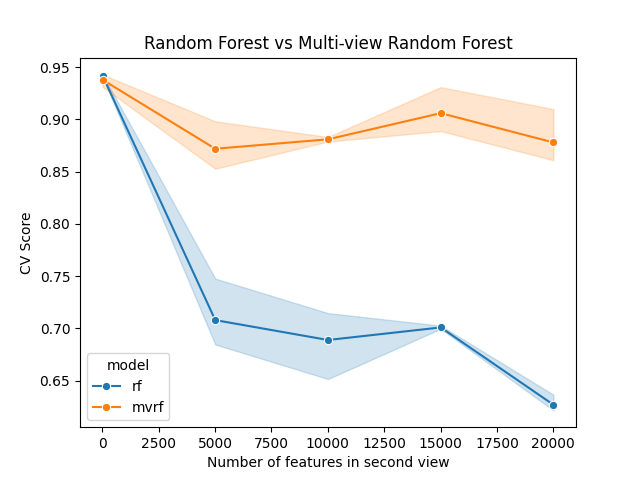
As we can see, the multi-view random forest outperforms the regular random forest as the number of features in the second view increases. This is because the multi-view random forest samples from each feature-set uniformly, while the regular random forest samples from all features uniformly. This is a key difference between the two forests.

Estimated memory usage: 914 MB