ExtendedIsolationForest example

An example using ExtendedIsolationForest for anomaly detection, which compares to the IsolationForest based on the algorithm in [1].

In the present example we demo two ways to visualize the decision boundary of an Extended Isolation Forest trained on a toy dataset.

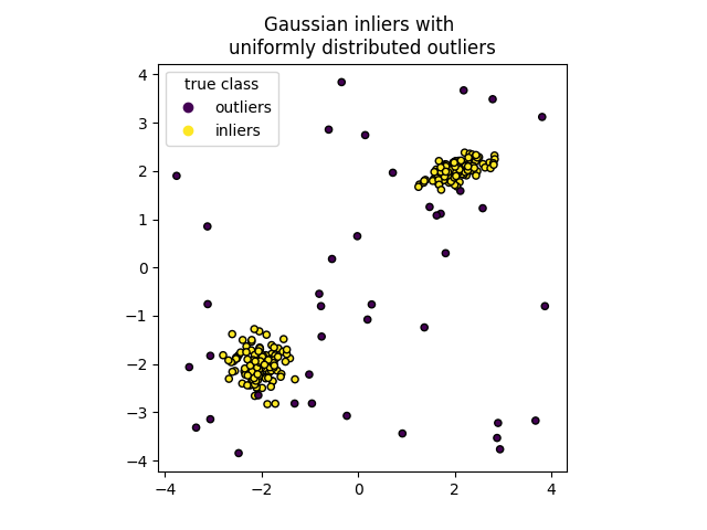
Data generation

We generate two clusters (each one containing n_samples) by randomly sampling the standard normal distribution as returned by numpy.random.randn(). One of them is spherical and the other one is slightly deformed.

For consistency with the IsolationForest notation, the inliers (i.e. the gaussian clusters) are assigned a ground truth label 1 whereas the outliers (created with numpy.random.uniform()) are assigned the label -1.

from copy import copy

import matplotlib.pyplot as plt
import numpy as np
from sklearn.ensemble import IsolationForest
from sklearn.inspection import DecisionBoundaryDisplay
from sklearn.model_selection import train_test_split

from treeple import ExtendedIsolationForest

n_samples, n_outliers = 120, 40
rng = np.random.RandomState(0)
covariance = np.array([[0.5, -0.1], [0.7, 0.4]])
cluster_1 = 0.4 * rng.randn(n_samples, 2) @ covariance + np.array([2, 2])  # general
cluster_2 = 0.3 * rng.randn(n_samples, 2) + np.array([-2, -2])  # spherical
outliers = rng.uniform(low=-4, high=4, size=(n_outliers, 2))

X = np.concatenate([cluster_1, cluster_2, outliers])
y = np.concatenate([np.ones((2 * n_samples), dtype=int), -np.ones((n_outliers), dtype=int)])

X_train, X_test, y_train, y_test = train_test_split(X, y, stratify=y, random_state=42)

We can visualize the resulting clusters:

scatter = plt.scatter(X[:, 0], X[:, 1], c=y, s=20, edgecolor="k")
handles, labels = scatter.legend_elements()
plt.axis("square")
plt.legend(handles=handles, labels=["outliers", "inliers"], title="true class")
plt.title("Gaussian inliers with \nuniformly distributed outliers")
plt.show()

Training of the model

extended_clf = ExtendedIsolationForest(max_samples=100, random_state=0, feature_combinations=2)
extended_clf.fit(X_train)

clf = IsolationForest(max_samples=100, random_state=0)
clf.fit(X_train)

IsolationForest(max_samples=100, random_state=0)

In a Jupyter environment, please rerun this cell to show the HTML representation or trust the notebook.
On GitHub, the HTML representation is unable to render, please try loading this page with nbviewer.org.

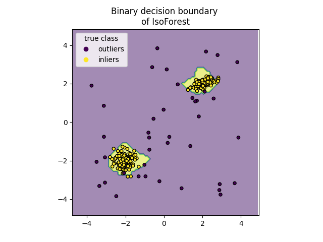
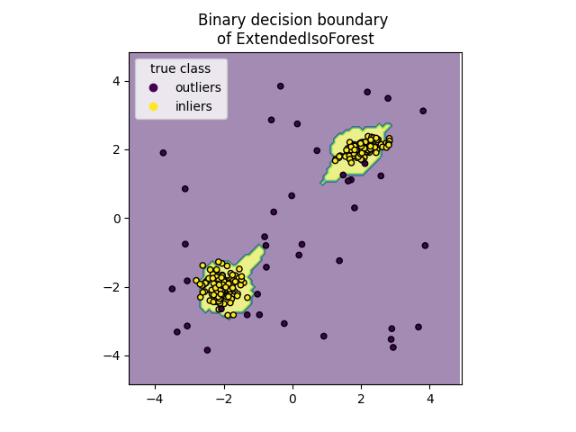
Plot discrete decision boundary

We use the class DecisionBoundaryDisplay to visualize a discrete decision boundary. The background color represents whether a sample in that given area is predicted to be an outlier or not. The scatter plot displays the true labels.

for name, model in zip(["IsoForest", "ExtendedIsoForest"], [clf, extended_clf]):
    disp = DecisionBoundaryDisplay.from_estimator(
        model,
        X,
        response_method="predict",
        alpha=0.5,
    )
    disp.ax_.scatter(X[:, 0], X[:, 1], c=y, s=20, edgecolor="k")
    disp.ax_.set_title(f"Binary decision boundary \nof {name}")
    plt.axis("square")
    plt.legend(handles=handles, labels=["outliers", "inliers"], title="true class")
    plt.show()

• 
• 

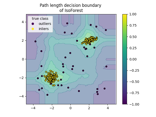
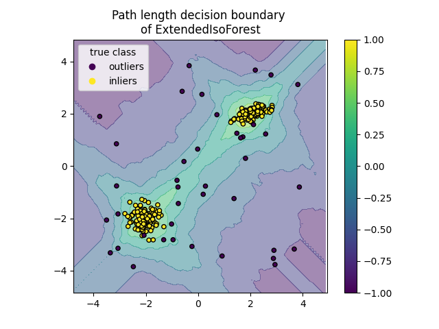
Plot path length decision boundary

By setting the response_method="decision_function", the background of the DecisionBoundaryDisplay represents the measure of normality of an observation. Such score is given by the path length averaged over a forest of random trees, which itself is given by the depth of the leaf (or equivalently the number of splits) required to isolate a given sample.

When a forest of random trees collectively produce short path lengths for isolating some particular samples, they are highly likely to be anomalies and the measure of normality is close to 0. Similarly, large paths correspond to values close to 1 and are more likely to be inliers.

for name, model in zip(["IsoForest", "ExtendedIsoForest"], [clf, extended_clf]):
    disp = DecisionBoundaryDisplay.from_estimator(
        model,
        X,
        response_method="decision_function",
        alpha=0.5,
    )
    disp.ax_.scatter(X[:, 0], X[:, 1], c=y, s=20, edgecolor="k")
    disp.ax_.set_title(f"Path length decision boundary \nof {name}")
    plt.axis("square")
    plt.legend(handles=handles, labels=["outliers", "inliers"], title="true class")
    plt.colorbar(disp.ax_.collections[1])
    plt.show()

• 
• 

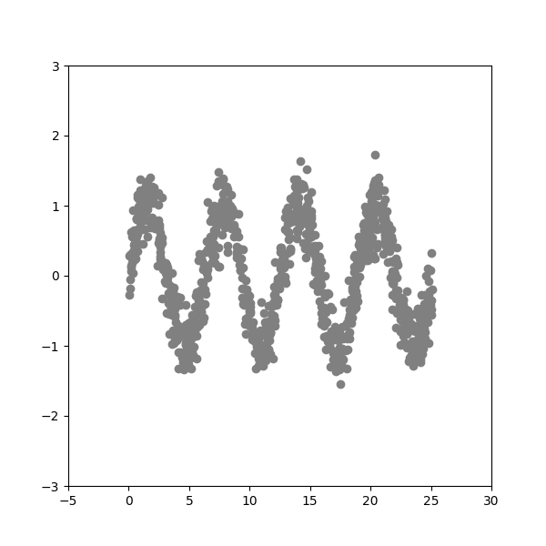
Generate Data Produce 2-D dataset with a sinusoidal shape and Gaussian noise added on top.

N = 1000
x = np.random.rand(N) * 8 * np.pi
y = np.sin(x) + np.random.randn(N) / 4.0
X = np.array([x, y]).T

fig = plt.figure(figsize=(6, 6))
fig.add_subplot(111)
plt.plot(X[:, 0], X[:, 1], "o", color=[0.5, 0.5, 0.5])

plt.xlim([-5, 30])
plt.ylim([-3.0, 3.0])

plt.show()

extended_clf = ExtendedIsolationForest(
    max_samples=100, random_state=0, n_estimators=200, feature_combinations=2
)
extended_clf.fit(X)

clf = IsolationForest(max_samples=100, random_state=0, n_estimators=200)
clf.fit(X)

IsolationForest(max_samples=100, n_estimators=200, random_state=0)

In a Jupyter environment, please rerun this cell to show the HTML representation or trust the notebook.
On GitHub, the HTML representation is unable to render, please try loading this page with nbviewer.org.

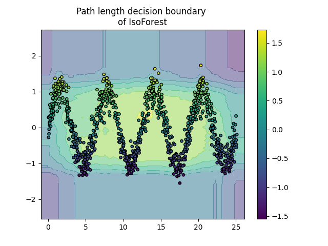
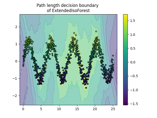
Plot discrete decision boundary

for name, model in zip(["IsoForest", "ExtendedIsoForest"], [clf, extended_clf]):
    disp = DecisionBoundaryDisplay.from_estimator(
        model,
        X,
        response_method="decision_function",
        alpha=0.5,
    )
    disp.ax_.scatter(X[:, 0], X[:, 1], c=y, s=15, edgecolor="k")
    disp.ax_.set_title(f"Path length decision boundary \nof {name}")
    plt.colorbar(disp.ax_.collections[1])
    plt.show()

• 
• 

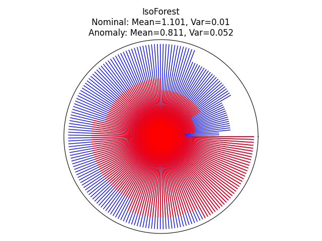
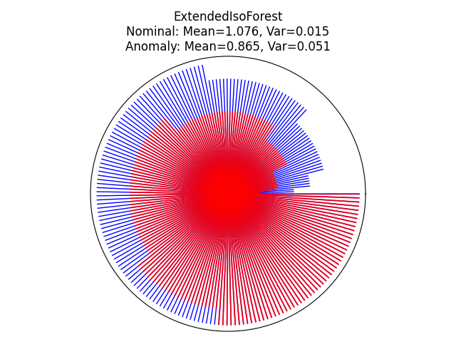
Visualize the prediction of each tree within the forest

We can visualize the prediction of each tree within the forest by using a circle plot and showing the depth at which each tree isolates a given sample. Here, we will evaluate two samples in the sinusoidal plot: one inlier and one outlier. The inlier is located at the center of the sinusoidal and the outlier is located at the bottom right corner of the plot.

inlier_sample = np.array([10.0, 0.0])
outlier_sample = np.array([-5.0, -3.0])

for name, model in zip(["IsoForest", "ExtendedIsoForest"], [clf, extended_clf]):
    theta = np.linspace(0, 2 * np.pi, len(model.estimators_))
    max_tree_depth = max([model.estimators_[i].get_depth() for i in range(len(model.estimators_))])

    fig = plt.figure()
    ax = plt.subplot(111, projection="polar")

    radii_in = []
    radii_out = []

    # get the depth of each samples
    for radii, sample, color, lw, alpha in zip(
        [radii_in, radii_out], [inlier_sample, outlier_sample], ["b", "r"], [1, 1.3], [1, 0.9]
    ):
        for i in range(len(model.estimators_)):
            # get the max depth of this tree
            max_depth_tree = model.estimators_[i].get_depth()

            leaf_index = model.estimators_[i].apply(sample.reshape(1, -1))
            # get the depth of each tree's leaf node for this sample
            depth = model._decision_path_lengths[i][leaf_index].squeeze()
            radii.append(depth)

        radii = np.array(radii)
        radii = np.sort(radii) / max_tree_depth
        for j in range(len(radii)):
            ax.plot([theta[j], theta[j]], [0, radii[j]], color=color, alpha=alpha, lw=lw)

        if color == "b":
            radii_in = copy(radii)
        else:
            radii_out = copy(radii)

    ax.set(
        title=f"{name}\nNominal: Mean={np.mean(radii_in).round(3)}, "
        f"Var={np.var(radii_in).round(3)}\n"
        f"Anomaly: Mean={np.mean(radii_out).round(3)}, Var={np.var(radii_out).round(3)}",
        xlabel="Anomaly",
    )
    ax.set_xticklabels([])
    ax.axes.get_xaxis().set_visible(False)
    ax.axes.get_yaxis().set_visible(False)
    fig.tight_layout()
    plt.show()

• 
• 

References

[1]

Sahand Hariri, Matias Carrasco Kind, and Robert J Brunner. Extended isolation forest. IEEE transactions on knowledge and data engineering, 33(4):1479–1489, 2019.

Estimated memory usage: 237 MB