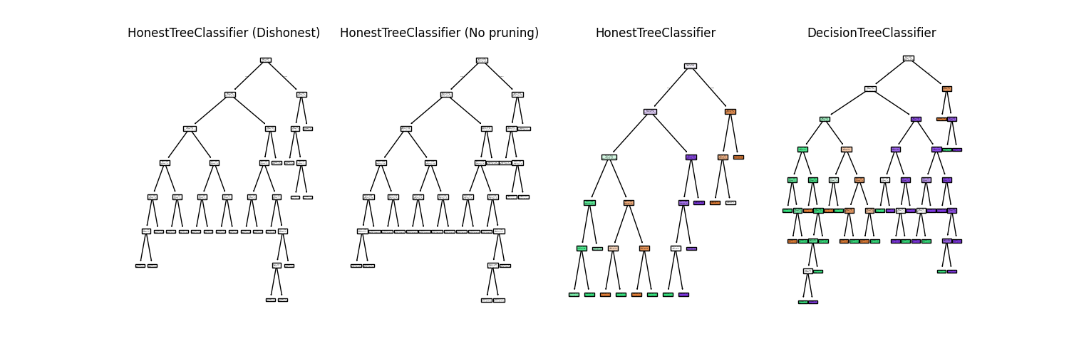
Comparison of Decision Tree and Honest Tree

This example compares the treeple.tree.HonestTreeClassifier from the treeple library with the sklearn.tree.DecisionTreeClassifier from scikit-learn on the Iris dataset.

Both classifiers are fitted on the same dataset and their decision trees are plotted side by side.

import matplotlib.pyplot as plt
from sklearn import config_context
from sklearn.datasets import load_iris
from sklearn.model_selection import train_test_split
from sklearn.tree import DecisionTreeClassifier, plot_tree

from treeple.tree import HonestTreeClassifier

# Load the iris dataset
iris = load_iris()
X, y = iris.data, iris.target
X_train, X_val, y_train, y_val = train_test_split(X, y, test_size=0.1, random_state=0)

# Initialize classifiers
max_features = 0.3

dishonest_clf = HonestTreeClassifier(
    honest_method=None,
    max_features=max_features,
    random_state=0,
    honest_prior="ignore",
)
honest_noprune_clf = HonestTreeClassifier(
    honest_method="apply",
    max_features=max_features,
    random_state=0,
    honest_prior="ignore",
)
honest_clf = HonestTreeClassifier(honest_method="prune", max_features=max_features, random_state=0)
sklearn_clf = DecisionTreeClassifier(max_features=max_features, random_state=0)

# Fit classifiers
dishonest_clf.fit(X_train, y_train)
honest_noprune_clf.fit(X_train, y_train)
honest_clf.fit(X_train, y_train)
sklearn_clf.fit(X_train, y_train)

# Plotting the trees
fig, axes = plt.subplots(nrows=1, ncols=4, figsize=(15, 5))

# .. note:: We skip parameter validation because internally the `plot_tree`
#           function checks if the estimator is a DecisionTreeClassifier
#           instance from scikit-learn, but the ``HonestTreeClassifier`` is
#           a subclass of a forked version of the DecisionTreeClassifier.

# Plot HonestTreeClassifier tree
ax = axes[2]
with config_context(skip_parameter_validation=True):
    plot_tree(honest_clf, filled=True, ax=ax)
ax.set_title("HonestTreeClassifier")

# Plot HonestTreeClassifier tree
ax = axes[1]
with config_context(skip_parameter_validation=True):
    plot_tree(honest_noprune_clf, filled=False, ax=ax)
ax.set_title("HonestTreeClassifier (No pruning)")

# Plot HonestTreeClassifier tree
ax = axes[0]
with config_context(skip_parameter_validation=True):
    plot_tree(dishonest_clf, filled=False, ax=ax)
ax.set_title("HonestTreeClassifier (Dishonest)")


# Plot scikit-learn DecisionTreeClassifier tree
plot_tree(sklearn_clf, filled=True, ax=axes[3])
axes[3].set_title("DecisionTreeClassifier")

plt.show()

Discussion

The HonestTreeClassifier is a variant of the DecisionTreeClassifier that provides honest inference. The honest inference is achieved by splitting the dataset into two parts: the training set and the validation set. The training set is used to build the tree, while the validation set is used to fit the leaf nodes for posterior prediction. This results in calibrated posteriors (see Plot honest forest calibrations on overlapping gaussian simulations).

Compared to the honest_prior='apply' method, the honest_prior='prune' method builds a tree that will not contain empty leaves, and also leverages the validation set to check split conditions. Thus we see that the pruned honest tree is significantly smaller than the regular decision tree.

Evaluate predictions of the trees

When we do not prune, note that the honest tree will have empty leaves that predict the prior. In this case, honest_prior='ignore' is used to ignore these leaves when computing the posteriors, which will result in a posterior that is np.nan.

# this is the same as a decision tree classifier that is trained on less data
print("\nDishonest posteriors: ", dishonest_clf.predict_proba(X_val))

# this is the honest tree with empty leaves that predict the prior
print("\nHonest tree without pruning: ", honest_noprune_clf.predict_proba(X_val))

# this is the honest tree that is pruned
print("\nHonest tree with pruning: ", honest_clf.predict_proba(X_val))

# this is a regular decision tree classifier from sklearn
print("\nDTC: ", sklearn_clf.predict_proba(X_val))

Dishonest posteriors:  [[0. 0. 1.]
 [0. 1. 0.]
 [1. 0. 0.]
 [0. 0. 1.]
 [1. 0. 0.]
 [0. 0. 1.]
 [1. 0. 0.]
 [0. 1. 0.]
 [0. 0. 1.]
 [0. 1. 0.]
 [0. 0. 1.]
 [0. 1. 0.]
 [0. 1. 0.]
 [0. 1. 0.]
 [0. 1. 0.]]

Honest tree without pruning:  [[       nan        nan        nan]
 [0.         1.         0.        ]
 [0.78571429 0.         0.21428571]
 [0.         0.         1.        ]
 [1.         0.         0.        ]
 [0.         0.         1.        ]
 [0.78571429 0.         0.21428571]
 [0.         1.         0.        ]
 [       nan        nan        nan]
 [0.         0.9        0.1       ]
 [0.         0.         1.        ]
 [0.         1.         0.        ]
 [0.         0.9        0.1       ]
 [0.         0.9        0.1       ]
 [0.         1.         0.        ]]

Honest tree with pruning:  [[0.         0.14285714 0.85714286]
 [0.25       0.75       0.        ]
 [1.         0.         0.        ]
 [0.         0.         1.        ]
 [1.         0.         0.        ]
 [0.         0.         1.        ]
 [1.         0.         0.        ]
 [0.         1.         0.        ]
 [0.         0.14285714 0.85714286]
 [0.         1.         0.        ]
 [0.         0.         1.        ]
 [0.         1.         0.        ]
 [0.         1.         0.        ]
 [0.         1.         0.        ]
 [0.33333333 0.66666667 0.        ]]

DTC:  [[0. 0. 1.]
 [0. 1. 0.]
 [1. 0. 0.]
 [0. 0. 1.]
 [1. 0. 0.]
 [0. 0. 1.]
 [1. 0. 0.]
 [0. 1. 0.]
 [0. 1. 0.]
 [0. 1. 0.]
 [0. 1. 0.]
 [0. 1. 0.]
 [0. 1. 0.]
 [0. 1. 0.]
 [0. 1. 0.]]

Estimated memory usage: 236 MB