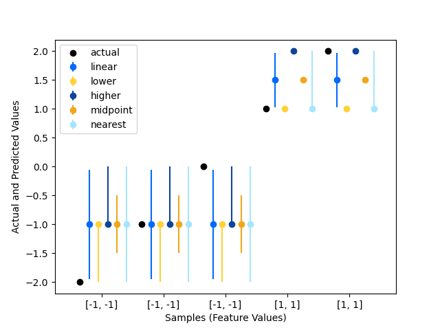
Predicting with different quantile interpolation methods

An example comparison of interpolation methods that can be applied during prediction when the desired quantile lies between two data points.

This example was heavily inspired by quantile-forest package. See their package here.

from collections import defaultdict

import matplotlib.pyplot as plt
import numpy as np
from sklearn.ensemble import RandomForestRegressor

Generate the data

We use four simple data points to illustrate the difference between the intervals that are generated using different interpolation methods.

X = np.array([[-1, -1], [-1, -1], [-1, -1], [1, 1], [1, 1]])
y = np.array([-2, -1, 0, 1, 2])

The interpolation methods

The following interpolation methods demonstrated here are: To interpolate between the data points, i and j (i <= j), linear, lower, higher, midpoint, or nearest. For more details, see treeple.RandomForestRegressor. The difference between the methods can be illustrated with the following example:

interpolations = ["linear", "lower", "higher", "midpoint", "nearest"]
colors = ["#006aff", "#ffd237", "#0d4599", "#f2a619", "#a6e5ff"]
quantiles = [0.025, 0.5, 0.975]

y_medians = []
y_errs = []
est = RandomForestRegressor(
    n_estimators=1,
    random_state=0,
)
# fit the model
est.fit(X, y)
# get the leaf nodes that each sample fell into
leaf_ids = est.apply(X)
# create a list of dictionary that maps node to samples that fell into it
# for each tree
node_to_indices = []
for tree in range(leaf_ids.shape[1]):
    d = defaultdict(list)
    for id, leaf in enumerate(leaf_ids[:, tree]):
        d[leaf].append(id)
    node_to_indices.append(d)
# drop the X_test to the trained tree and
# get the indices of leaf nodes that fall into it
leaf_ids_test = est.apply(X)
# for each samples, collect the indices of the samples that fell into
# the same leaf node for each tree
y_pred_quantile = []
for sample in range(leaf_ids_test.shape[0]):
    li = [
        node_to_indices[tree][leaf_ids_test[sample][tree]] for tree in range(leaf_ids_test.shape[1])
    ]
    # merge the list of indices into one
    idx = [item for sublist in li for item in sublist]
    # get the y_train for each corresponding id``
    y_pred_quantile.append(y[idx])

for interpolation in interpolations:
    # get the quatile preditions for each predicted sample
    y_pred = [
        np.array(
            [
                np.quantile(y_pred_quantile[i], quantile, method=interpolation)
                for i in range(len(y_pred_quantile))
            ]
        )
        for quantile in quantiles
    ]
    y_medians.append(y_pred[1])
    y_errs.append(
        np.concatenate(
            (
                [y_pred[1] - y_pred[0]],
                [y_pred[2] - y_pred[1]],
            ),
            axis=0,
        )
    )

sc = plt.scatter(np.arange(len(y)) - 0.35, y, color="k", zorder=10)
ebs = []
for i, (median, y_err) in enumerate(zip(y_medians, y_errs)):
    ebs.append(
        plt.errorbar(
            np.arange(len(y)) + (0.15 * (i + 1)) - 0.35,
            median,
            yerr=y_err,
            color=colors[i],
            ecolor=colors[i],
            fmt="o",
        )
    )
plt.xlim([-0.75, len(y) - 0.25])
plt.xticks(np.arange(len(y)), X.tolist())
plt.xlabel("Samples (Feature Values)")
plt.ylabel("Actual and Predicted Values")
plt.legend([sc] + ebs, ["actual"] + interpolations, loc=2)
plt.show()

Estimated memory usage: 227 MB