Quantile prediction with Random Forest Regressor class

An example that demonstrates how to use the Random Forest to generate quantile predictions such as conditional median and prediction intervals. The example compares the predictions to a ground truth function used to generate noisy samples.

This example was heavily inspired by quantile-forest package. See their package here.

from collections import defaultdict

import matplotlib.pyplot as plt
import numpy as np
from sklearn.ensemble import RandomForestRegressor
from sklearn.model_selection import train_test_split

Generate the data

def make_toy_dataset(n_samples, seed=0):
    rng = np.random.RandomState(seed)

    x = rng.uniform(0, 10, size=n_samples)
    f = x * np.sin(x)

    sigma = 0.25 + x / 10
    noise = rng.lognormal(sigma=sigma) - np.exp(sigma**2 / 2)
    y = f + noise

    return np.atleast_2d(x).T, y


n_samples = 1000
X, y = make_toy_dataset(n_samples)

X_train, X_test, y_train, y_test = train_test_split(X, y, random_state=0)

xx = np.atleast_2d(np.linspace(0, 10, n_samples)).T

Fit the model to the training samples

rf = RandomForestRegressor(max_depth=3, random_state=0)
rf.fit(X_train, y_train)

y_pred = rf.predict(xx)

# get the leaf nodes that each sample fell into
leaf_ids = rf.apply(X_train)
# create a list of dictionary that maps node to samples that fell into it
# for each tree
node_to_indices = []
for tree in range(leaf_ids.shape[1]):
    d = defaultdict(list)
    for id, leaf in enumerate(leaf_ids[:, tree]):
        d[leaf].append(id)
    node_to_indices.append(d)
# drop the X_test to the trained tree and
# get the indices of leaf nodes that fall into it
leaf_ids_test = rf.apply(xx)
# for each samples, collect the indices of the samples that fell into
# the same leaf node for each tree
y_pred_quatile = []
for sample in range(leaf_ids_test.shape[0]):
    li = [
        node_to_indices[tree][leaf_ids_test[sample][tree]] for tree in range(leaf_ids_test.shape[1])
    ]
    # merge the list of indices into one
    idx = [item for sublist in li for item in sublist]
    # get the y_train for each corresponding id
    y_pred_quatile.append(y_train[idx])
# get the quatile preditions for each predicted sample
y_pred_low = [np.quantile(y_pred_quatile[i], 0.025) for i in range(len(y_pred_quatile))]
y_pred_med = [np.quantile(y_pred_quatile[i], 0.5) for i in range(len(y_pred_quatile))]
y_pred_upp = [np.quantile(y_pred_quatile[i], 0.975) for i in range(len(y_pred_quatile))]

Plot the results

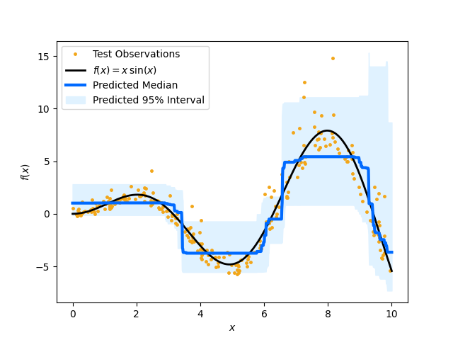
Plot the conditional median and prediction intervals. The blue line is the predicted median and the shaded area indicates the 95% confidence interval of the prediction. The dots are the training data and the black line indicates the function that is used to generated those samples.

plt.plot(X_test, y_test, ".", c="#f2a619", label="Test Observations", ms=5)
plt.plot(xx, (xx * np.sin(xx)), c="black", label="$f(x) = x\,\sin(x)$", lw=2)
plt.plot(xx, y_pred_med, c="#006aff", label="Predicted Median", lw=3, ms=5)
plt.fill_between(
    xx.ravel(),
    y_pred_low,
    y_pred_upp,
    color="#e0f2ff",
    label="Predicted 95% Interval",
)
plt.xlabel("$x$")
plt.ylabel("$f(x)$")
plt.legend(loc="upper left")
plt.show()

Estimated memory usage: 326 MB