One-sample feedforwardness testing: simulation¶

Preliminaries¶

from pkg.utils import set_warnings

import datetime
import time

import matplotlib.pyplot as plt
import numpy as np
import pandas as pd
import seaborn as sns

from graspologic.plot import heatmap
from graspologic.simulations import sample_edges, sbm
from graspologic.utils import remove_loops
from pkg.flow import rank_graph_match_flow
from pkg.io import savefig
from pkg.plot import set_theme

set_warnings()

np.random.seed(8888)

t0 = time.time()


def stashfig(name, **kwargs):
    foldername = "feedforwardness_sims"
    savefig(name, foldername=foldername, **kwargs)


colors = sns.color_palette("Set1")
set_theme()

A test for feedforwardness¶

We’ll use the simple model above to motivate a one-sided test for feedforwardness as follows:

\[ H_0: p_{upper} = p_{lower} = p \]

\[ H_A: p_{upper} > p_{lower} \]

A test statistic for feedforwardness¶

We aim to perform a 1-sample test for \(H_0\) vs \(H_a\). The test statistic we use is simply \(\hat{p}_{upper}\), the proportion of edges in the upper triangle. To estimate this test statistic from a network, we use graph matching to try to maximize the proportion of edges in the upper triangle (see this notebook for an application of this idea to team ranking).

TODO: some visual explanation of our test statistic¶

Evaluating the test for different models of feedforwardness¶

The upset model¶

This model is one of the simplest feedforward models we can think of. This model is parameterized by two probabilities and a ranking/permutation of a set of nodes.

Let the feedforward probability be \(p_{fwd}\), and let the feedback probability be \(p_{back}\). Assume we have a permutation of the nodes described by the vector of integers \(\phi \in \mathbb{R}^n\), where \(n\) is the number of nodes. Each element of \(\phi\) is the node’s “rank” in the network, which, along with the probabilities above, determine its probability of connecting to other nodes in the network. Thus, each element of \(\phi\) is a unique integer \(\in \{ 0 ... n - 1\}\).

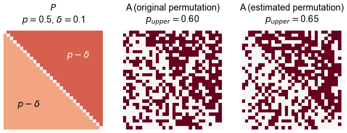
If we sort \(P\) according to \(\phi\) (largest to smallest) then \(P\) looks as follows:

\[\begin{split} P_{ij} = \begin{cases} p_{fwd} & i < j \\ p_{back} & i > j \\ 0 & i = j \\ \end{cases} \end{split}\]

Thus, \(P\) has all \(p_{fwd}\) on the upper triangle, and all \(p_{back}\) on the lower triangle. Note that this can equivalently be parameterized as

\[ p = \frac{p_{fwd} + p_{back}}{2} \quad \delta = \frac{p_{fwd} - p_{back}}{2} \]

Under this parameterization, \(\delta \in [0, 0.5]\) can be thought of as how feedforward the network is - high values mean feedforward edges are far much more likely, and thus the network structure respects the ranking \(\phi\) more. \(p\) then just sets the overall density of the network.

def calculate_p_upper(A):
    A = remove_loops(A)
    n = len(A)
    triu_inds = np.triu_indices(n, k=1)
    upper_triu_sum = A[triu_inds].sum()
    total_sum = A.sum()
    upper_triu_p = upper_triu_sum / total_sum
    return upper_triu_p


def construct_feedforward_P(n, p=0.5, delta=0):
    triu_inds = np.triu_indices(n, k=1)
    p_upper = p + delta
    p_lower = p - delta
    P = np.zeros((n, n))
    P[triu_inds] = p_upper
    P[triu_inds[::-1]] = p_lower
    return P


n = 30
p = 0.5
delta = 0.1

P = construct_feedforward_P(n, p=p, delta=delta)

A = sample_edges(P, directed=True, loops=False)

fig, axs = plt.subplots(1, 3, figsize=(12, 4))

# TODO make a plot of Phat
title = r"$P$" + "\n"
title += r"$p = $" + f"{p}, " + r"$\delta = $" + f"{delta}"
ax = axs[0]
heatmap(P, vmin=0, vmax=1, cbar=False, ax=ax, title=title)
ax.text(n / 4, 3 * n / 4, r"$p - \delta$", ha="center", va="center")
ax.text(3 * n / 4, n / 4, r"$p - \delta$", ha="center", va="center", color="white")

p_upper = calculate_p_upper(A)
title = "A (original permutation)\n"
title += r"$p_{upper} = $" + f"{p_upper:0.2f}"
heatmap(A, cbar=False, ax=axs[1], title=title)

perm_inds = rank_graph_match_flow(A)
p_upper = calculate_p_upper(A[np.ix_(perm_inds, perm_inds)])

title = "A (estimated permutation)\n"
title += r"$p_{upper} = $" + f"{p_upper:0.2f}"
heatmap(A[np.ix_(perm_inds, perm_inds)], cbar=False, ax=axs[2], title=title)

<AxesSubplot:title={'center':'A (estimated permutation)\n$p_{upper} = $0.65'}>

Simulate from the null¶

Here, we set

\[\begin{split} p = 0.5\\ n = 30\\ \delta = 0 \end{split}\]

After sampling each network we compute the test statistic above, and collect these test statistics for our null distribution.

def sample_null_distribution(sample_func, tstat_func, n_samples=1000, print_time=True):
    null = []
    currtime = time.time()
    for i in range(n_samples):
        A = sample_func()
        tstat = tstat_func(A)
        null.append(tstat)
    if print_time:
        print(f"{time.time() - currtime:.3f} seconds elapsed.")
    null = np.array(null)
    null = np.sort(null)
    return null


def sample_upset():
    P = construct_feedforward_P(n, p=p, delta=0)
    A = sample_edges(P, directed=True, loops=False)
    return A


def p_upper_tstat(A):
    perm_inds = rank_graph_match_flow(A)
    p_upper = calculate_p_upper(A[np.ix_(perm_inds, perm_inds)])
    return p_upper


null = sample_null_distribution(sample_upset, p_upper_tstat)

30.464 seconds elapsed.

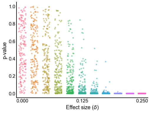
Simulate from the alternative and test for feedforwardness¶

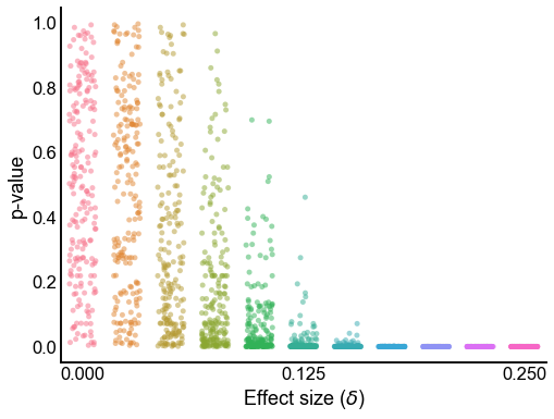
Here, we let the “amount of feedforwardness”, \(\delta\), vary from 0 to 0.25. \(\delta\) can be interpreted as the effect size. For each \(\delta\) we sample 200 graphs, and run a test for feedforwardness. The test computes the test statistic described above, and then compares to the bootstrapped null distribution we computed above to calculate a p-value.

Note that here I am calculating p-values using the same null distribution for all of these tests (for now, just for simplicity). This assumes that the parameter \(p\) is known, thus we only need to estimate \(\delta\). In real data we would have to use the plug in estimate of \(\hat{p}\) which is the ER global connection probability that we’d estimate from the data (i.e. \(\frac{M}{N (N - 1)}\)), and then we’d sample networks from that model to generate our bootstrap null distribution.

Also note that there are plenty of other reasonable null models we could use to generate our null distribution, including degree-corrected ER.

def compute_statistics(A, null):
    row = {}
    row["sampled_p_upper"] = calculate_p_upper(A)
    p_upper = p_upper_tstat(A)
    row["estimated_p_upper"] = p_upper
    row["estimated_p"] = np.sum(A) / (A.size - len(A))
    ind = np.searchsorted(null, p_upper)
    row["pvalue"] = 1 - ind / len(
        null
    )  # TODO make more exact but this is roughly right
    return row


deltas = np.linspace(0, 0.25, num=11)
n_samples = 200
rows = []
currtime = time.time()
for delta in deltas:
    P = construct_feedforward_P(n, p=p, delta=delta)
    for i in range(n_samples):
        row = {}
        # sample
        A = sample_edges(P, directed=True, loops=False)
        row = compute_statistics(A, null)
        row["delta"] = delta
        row["str_delta"] = f"{delta:0.3f}"
        rows.append(row)
print(f"{time.time() - currtime:.3f} seconds elapsed.")

results = pd.DataFrame(rows)

65.485 seconds elapsed.

Create a color map¶

str_deltas = np.unique(results["str_delta"])
colors = sns.color_palette("husl", len(str_deltas))
palette = dict(zip(str_deltas, colors))
for i, d in enumerate(str_deltas):
    palette[float(d)] = colors[i]

Plot the p-values from varying effect sizes¶

def plot_pvalues(results):
    fig, ax = plt.subplots(1, 1, figsize=(8, 6))
    sns.stripplot(
        data=results,
        x="str_delta",
        y="pvalue",
        hue="str_delta",
        palette=palette,
        zorder=2,
        alpha=0.5,
        jitter=0.3,
    )
    ax.get_legend().remove()
    ax.set(xlabel=r"Effect size ($\delta$)", ylabel="p-value")
    ax.xaxis.set_major_locator(plt.FixedLocator([0, 5, 10]))
    return ax


plot_pvalues(results)

<AxesSubplot:xlabel='Effect size ($\\delta$)', ylabel='p-value'>

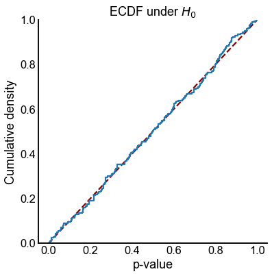
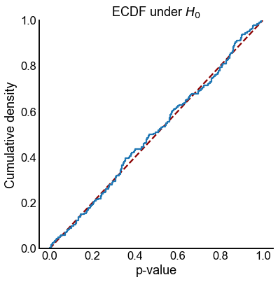
Plot the distribution p-values under the null¶

def plot_null_ecdf(results):
    fig, ax = plt.subplots(1, 1, figsize=(6, 6))
    sns.ecdfplot(data=results[results["str_delta"] == "0.000"], x="pvalue")
    ax.set(xlabel="p-value", ylabel="Cumulative density", title=r"ECDF under $H_0$")
    ax.plot([0, 1], [0, 1], color="darkred", linestyle="--", zorder=-1)
    return ax


plot_null_ecdf(results)

<AxesSubplot:title={'center':'ECDF under $H_0$'}, xlabel='p-value', ylabel='Cumulative density'>

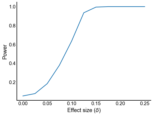
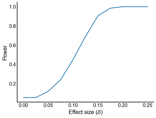
Plot power for \(\alpha = 0.05\)¶

def calc_power_at(x, alpha=0.05):
    return (x < alpha).sum() / len(x)


def plot_power(results):
    grouped_results = results.groupby("str_delta")
    power = grouped_results["pvalue"].agg(calc_power_at)
    power.name = "power"
    power = power.to_frame().reset_index()
    power["delta"] = power["str_delta"].astype(float)
    fig, ax = plt.subplots(1, 1, figsize=(8, 6))
    sns.lineplot(data=power, x="delta", y="power", ax=ax)
    ax.set(ylabel="Power", xlabel=r"Effect size ($\delta$)")
    return ax


plot_power(results)

<AxesSubplot:xlabel='Effect size ($\\delta$)', ylabel='Power'>

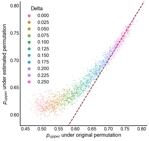
Plot the “true” and estimated upper triangle probabilities¶

By true upper triangle probabilies, we mean the proportion of edges in the upper triangle under the permutation that we sampled the graph from, \(\phi\). The estimated upper triangle probability is what we estimate after permuting the network using graph matching.

Note that it may be possible to permute a network from its starting permutation \(\phi\) to make even more edges in the upper triangle. Conversely, it’s possible that graph matching fails to find a permutation with as many upper triangular edges as the original permutation (which we of course wouldn’t know on real data).

fig, ax = plt.subplots(1, 1, figsize=(8, 8))
sns.scatterplot(
    data=results,
    x="sampled_p_upper",
    y="estimated_p_upper",
    hue="str_delta",
    s=8,
    alpha=0.4,
    linewidth=0,
    ax=ax,
    zorder=10,
    palette=palette,
)
ax.get_legend().set_title("Delta")
plt.autoscale(False)
ax.plot([0, 1], [0, 1], color="darkred", linestyle="--", zorder=-1)
ax.set(
    xlabel=r"$p_{upper}$ under original permutation",
    ylabel=r"$p_{upper}$ under estimated permutation",
)

[Text(0.5, 0, '$p_{upper}$ under original permutation'),
 Text(0, 0.5, '$p_{upper}$ under estimated permutation')]

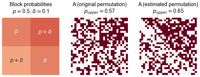
A feedforward SBM model¶

Here we construct a 2-block SBM where the block probabilities are feedforward with an amount that depends on \(\delta\).

def construct_feedforward_B(p=0.5, delta=0):
    B = np.array([[p, p + delta], [p - delta, p]])
    return B


delta = 0.1
B = construct_feedforward_B(0.5, delta)
ns = [15, 15]
A, labels = sbm(ns, B, directed=True, loops=False, return_labels=True)
fig, axs = plt.subplots(1, 3, figsize=(12, 4))

title = "Block probabilities\n"
title += r"$p = $" + f"{p}, " + r"$\delta = $" + f"{delta}"
annot = np.array([[r"$p$", r"$p + \delta$"], [r"$p + \delta$", r"$p$"]])
sns.heatmap(
    B,
    vmin=0,
    center=0,
    vmax=1,
    cmap="RdBu_r",
    annot=annot,
    cbar=False,
    square=True,
    fmt="",
    ax=axs[0],
    xticklabels=False,
    yticklabels=False,
)
axs[0].set_title(title, pad=16.5)

p_upper = calculate_p_upper(A)
title = "A (original permutation)\n"
title += r"$p_{upper} = $" + f"{p_upper:0.2f}"
heatmap(A, cbar=False, ax=axs[1], title=title)

perm_inds = rank_graph_match_flow(A)
p_upper = calculate_p_upper(A[np.ix_(perm_inds, perm_inds)])

title = "A (estimated permutation)\n"
title += r"$p_{upper} = $" + f"{p_upper:0.2f}"
heatmap(A[np.ix_(perm_inds, perm_inds)], cbar=False, ax=axs[2], title=title)

<AxesSubplot:title={'center':'A (estimated permutation)\n$p_{upper} = $0.65'}>

Simulate from the null¶

B = construct_feedforward_B(0.5, 0)

def sample_func():
    return sbm(ns, B, directed=True, loops=False)

null = sample_null_distribution(sample_func, p_upper_tstat)

29.691 seconds elapsed.

Simulate from the alternative and test for feedforwardness¶

deltas = np.linspace(0, 0.25, num=11)
n_samples = 200
rows = []
currtime = time.time()
for delta in deltas:
    B = construct_feedforward_B(p, delta)
    for i in range(n_samples):
        row = {}
        # sample
        A = sbm(ns, B, directed=True, loops=False)
        row = compute_statistics(A, null)
        row["delta"] = delta
        row["str_delta"] = f"{delta:0.3f}"
        rows.append(row)
print(f"{time.time() - currtime:.3f} seconds elapsed.")

results = pd.DataFrame(rows)

64.146 seconds elapsed.

Plot the p-values from varying effect sizes¶

plot_pvalues(results)

<AxesSubplot:xlabel='Effect size ($\\delta$)', ylabel='p-value'>

Plot the distribution p-values under the null¶

plot_null_ecdf(results)

<AxesSubplot:title={'center':'ECDF under $H_0$'}, xlabel='p-value', ylabel='Cumulative density'>

Plot power for \(\alpha = 0.05\)¶

plot_power(results)

<AxesSubplot:xlabel='Effect size ($\\delta$)', ylabel='Power'>

End¶

elapsed = time.time() - t0
delta = datetime.timedelta(seconds=elapsed)
print("----")
print(f"Script took {delta}")
print(f"Completed at {datetime.datetime.now()}")
print("----")

----
Script took 0:03:14.758523
Completed at 2021-03-24 14:25:22.496200
----

Maggot Connectome

One-sample feedforwardness testing: simulation¶

Preliminaries¶

A test for feedforwardness¶

A test statistic for feedforwardness¶

TODO: some visual explanation of our test statistic¶

Evaluating the test for different models of feedforwardness¶

The upset model¶

Simulate from the null¶

Simulate from the alternative and test for feedforwardness¶

Create a color map¶

Plot the p-values from varying effect sizes¶

Plot the distribution p-values under the null¶

Plot power for \(\alpha = 0.05\)¶

Plot the “true” and estimated upper triangle probabilities¶

A feedforward SBM model¶

Simulate from the null¶

Simulate from the alternative and test for feedforwardness¶

Plot the p-values from varying effect sizes¶

Plot the distribution p-values under the null¶

Plot power for \(\alpha = 0.05\)¶

End¶