A priori SBMs
Comparing connectivity models generated from biological node metadata
Problem statement
We are given an adjacency matrix \(A\) with \(n\) nodes, and a set of node metadata. Consider the \(p\)th “column” of the node metadata to be an \(n\)-length vector:
which represents a partition of the nodes into \(K^{(p)}\) groups.
We aim to understand which of these partitions are “good” at describing the connectivity we see in the network - for our purposes (for now), we will understand “good” in terms of the stochastic block model. One natural notion of “good” is a high likelihood of the observed network under the parameters fit for the stochastic block model using partition \(\tau^{(p)}\). However, using the likelihood alone would not balance how well our model fits the network with the complexity of the model - note that for a partition where each node is in its own partition, we could fit the data perfectly.
Thus, we consider notions of a tradeoff between model fit (likelihood) and complexity (the dimension of the parameter space associated with the model). Here we will use the Bayesian Information Criterion (BIC). Since \(\tau\) is fixed and not estimated from the data, the only parameters we need to estimate for the SBM are the elements of \(B\), a \(K^{(p)} \times K^{(p)}\) matrix of block probabilities. If we make no other assumptions about \(B\) (e.g. low-rank, planned partition), then there are \(K^{(p)}\) parameters we have to estimate in \(B\). Since we observe \(n^2\) edges/non-edges from \(A\), then BIC takes the form:
Below, we fit SBM models to the (unweighted) maggot connectome, using several metadata columns (as well as their intersections, explained below) as our partitions. We evaluate each in terms of BIC as described above.
from pkg.utils import set_warnings

set_warnings()

from itertools import chain, combinations
import os

import ipynb_path
import matplotlib.pyplot as plt
import networkx as nx
import numpy as np
import pandas as pd
import seaborn as sns
from mpl_toolkits.axes_grid1 import make_axes_locatable

from graspologic.models import SBMEstimator
from graspologic.plot import adjplot
from graspologic.utils import binarize, remove_loops
from pkg.data import load_adjacency, load_networkx, load_node_meta, load_palette
from pkg.plot import set_theme
from pkg.io import savefig


def stashfig(name, **kwargs):
    # get name of current script
    # try:
    #     filename = __file__
    # except:
    #     filename = ipynb_path.get()
    # foldername = os.path.basename(filename)[:-3]
    foldername = "a_priori_sbm"
    savefig(name, foldername=foldername, **kwargs)


def group_repr(group_keys):
    """Get a string representation of a list of group keys"""
    if len(group_keys) == 0:
        return "{}"
    elif len(group_keys) == 1:
        return str(group_keys[0])
    else:
        out = f"{group_keys[0]}"
        for key in group_keys[1:]:
            out += " x "
            out += key
        return out


def powerset(iterable, ignore_empty=True):
    # REF: https://stackoverflow.com/questions/1482308/how-to-get-all-subsets-of-a-set-powerset
    "powerset([1,2,3]) --> (1,) (2,) (3,) (1,2) (1,3) (2,3) (1,2,3)"
    s = list(iterable)
    return list(
        chain.from_iterable(combinations(s, r) for r in range(ignore_empty, len(s) + 1))
    )


def plot_upset_indicators(
    intersections,
    ax=None,
    facecolor="black",
    element_size=None,
    with_lines=True,
    horizontal=True,
    height_pad=0.7,
):
    # REF: https://github.com/jnothman/UpSetPlot/blob/e6f66883e980332452041cd1a6ba986d6d8d2ae5/upsetplot/plotting.py#L428
    """Plot the matrix of intersection indicators onto ax"""
    data = intersections
    n_cats = data.index.nlevels

    idx = np.flatnonzero(data.index.to_frame()[data.index.names].values)
    c = np.array(["lightgrey"] * len(data) * n_cats, dtype="O")
    c[idx] = facecolor
    x = np.repeat(np.arange(len(data)), n_cats)
    y = np.tile(np.arange(n_cats), len(data))
    if element_size is not None:
        s = (element_size * 0.35) ** 2
    else:
        # TODO: make s relative to colw
        s = 200
    ax.scatter(x, y, c=c.tolist(), linewidth=0, s=s)

    if with_lines:
        line_data = (
            pd.Series(y[idx], index=x[idx]).groupby(level=0).aggregate(["min", "max"])
        )
        ax.vlines(
            line_data.index.values,
            line_data["min"],
            line_data["max"],
            lw=2,
            colors=facecolor,
        )

    tick_axis = ax.yaxis
    tick_axis.set_ticks(np.arange(n_cats))
    tick_axis.set_ticklabels(data.index.names, rotation=0 if horizontal else -90)
    # ax.xaxis.set_visible(False)
    ax.tick_params(axis="both", which="both", length=0)
    if not horizontal:
        ax.yaxis.set_ticks_position("top")
    ax.set_frame_on(False)
    ax.set_ylim((-height_pad, n_cats - 1 + height_pad))


def upset_stripplot(data, x=None, y=None, ax=None, upset_ratio=0.3, **kwargs):
    divider = make_axes_locatable(ax)

    sns.stripplot(data=data, x=x, y=y, ax=ax, **kwargs)
    ax.set(xticks=[], xticklabels=[], xlabel="")

    upset_ax = divider.append_axes(
        "bottom", size=f"{upset_ratio*100}%", pad=0, sharex=ax
    )
    plot_upset_indicators(data, ax=upset_ax)
    upset_ax.set_xlabel("Grouping")
    return ax, upset_ax


palette = load_palette()
set_theme()
Load the data
Load node metadata and select the graph of interest
meta = load_node_meta()
meta = meta[meta["paper_clustered_neurons"]]

#%%[markdown]
# ### Create some new metadata columns from existing information
# make some new metadata columns
assert (
    meta[["ipsilateral_axon", "contralateral_axon", "bilateral_axon"]].sum(axis=1).max()
    == 1
)

meta["axon_lat"] = "other"
meta.loc[meta[meta["ipsilateral_axon"]].index, "axon_lat"] = "ipsi"
meta.loc[meta[meta["contralateral_axon"]].index, "axon_lat"] = "contra"
meta.loc[meta[meta["bilateral_axon"]].index, "axon_lat"] = "bi"

# TODO:
# io: input/"interneuron"/output
# probably others, need to think...
Load the graph
g = load_networkx(graph_type="G", node_meta=meta)
adj = nx.to_numpy_array(g, nodelist=meta.index)
adj = binarize(adj)
Fit a series of a priori SBMs
Here we use these known groupings of neurons to fit different a priori SBMs. As an
example, consider the groupings hemisphere and axon_lat. hemisphere indicates
whether a neuron is on the left, right, or center. axon_lat indicates whether a
neuron’s axon is ipsilateral, bilateral, or contralateral. We could fit an SBM
using either of these groupings as our partition of the nodes, but we could also use
hemisphere cross axon_lat to get categories like (left, ipsilateral),
(left, contralateral), etc.
Below, we fit SBMs using a variety of these different groupings. We evaluate each model in terms of log-likelihood, the number of parameters, and BIC.
single_group_keys = ["hemisphere", "simple_group", "lineage", "axon_lat"]
all_group_keys = powerset(single_group_keys, ignore_empty=False)

rows = []
for group_keys in all_group_keys:
    group_keys = list(group_keys)
    print(group_keys)

    if len(group_keys) > 0:
        # this is essentially just grabbing the labels that are group_key1 cross group_key2
        # etc. and then applying this as a column in the metadata
        groupby = meta.groupby(group_keys)
        groups = groupby.groups
        unique_group_keys = list(sorted(groups.keys()))
        group_map = dict(zip(unique_group_keys, range(len(unique_group_keys))))
        if len(group_keys) > 1:
            meta["_group"] = list(meta[group_keys].itertuples(index=False, name=None))
        else:
            meta["_group"] = meta[group_keys]
        meta["_group_id"] = meta["_group"].map(group_map)
    else:  # then this is the ER model...
        meta["_group_id"] = np.zeros(len(meta))

    # fitting the simple SBM
    Model = SBMEstimator
    estimator = Model(directed=True, loops=False)
    estimator.fit(adj, y=meta["_group_id"].values)

    # evaluating and saving results
    estimator.n_verts = len(adj)
    bic = estimator.bic(adj)
    lik = estimator.score(adj)
    n_params = estimator._n_parameters()
    penalty = 2 * np.log(len(adj)) * n_params
    row = {
        "bic": -bic,
        "lik": lik,
        "group_keys": group_repr(group_keys),
        "n_params": n_params,
        "penalty": penalty,
    }
    for g in single_group_keys:
        if g in group_keys:
            row[g] = True
        else:
            row[g] = False
    rows.append(row)
[]
['hemisphere']
['simple_group']
['lineage']
['axon_lat']
['hemisphere', 'simple_group']
['hemisphere', 'lineage']
['hemisphere', 'axon_lat']
['simple_group', 'lineage']
['simple_group', 'axon_lat']
['lineage', 'axon_lat']
['hemisphere', 'simple_group', 'lineage']
['hemisphere', 'simple_group', 'axon_lat']
['hemisphere', 'lineage', 'axon_lat']
['simple_group', 'lineage', 'axon_lat']
['hemisphere', 'simple_group', 'lineage', 'axon_lat']
Collect experimental results
results = pd.DataFrame(rows)
results.sort_values("bic", ascending=False, inplace=True)
results["rank"] = np.arange(len(results), 0, -1)
results = results.set_index(single_group_keys)
Evaluate model fits
Plot BIC, likelihood, and the number of parameters for each model
colors = sns.cubehelix_palette(
start=0.5, rot=-0.5, n_colors=results["group_keys"].nunique()
)[::-1]
palette = dict(zip(results["group_keys"].unique(), colors))
stripplot_kws = dict(
jitter=0,
x="group_keys",
s=10,
palette=palette,
upset_ratio=0.35,
)
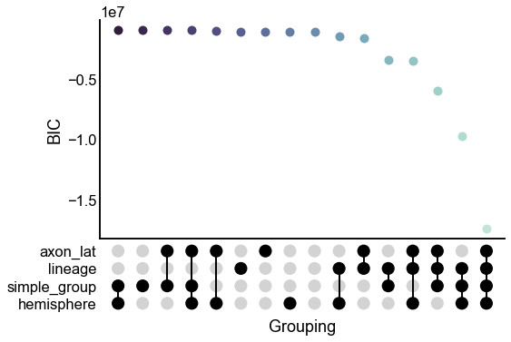
fig, ax = plt.subplots(1, 1, figsize=(8, 6))
upset_stripplot(results, y="bic", ax=ax, **stripplot_kws)
ax.set(ylabel="BIC")
stashfig("all-model-bic")
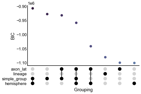
fig, ax = plt.subplots(1, 1, figsize=(8, 6))
upset_stripplot(results.iloc[:8], y="bic", ax=ax, **stripplot_kws)
ax.set(ylabel="BIC")
stashfig("first-8-model-bic")
# looked bad after switching to "maximize BIC" version
# fig, ax = plt.subplots(1, 1, figsize=(8, 6))
# upset_stripplot(results, y="bic", ax=ax, **stripplot_kws)
# ax.set(ylabel="BIC")
# ax.set_yscale("symlog")
# stashfig("all-model-bic-logy")
fig, ax = plt.subplots(1, 1, figsize=(8, 6))
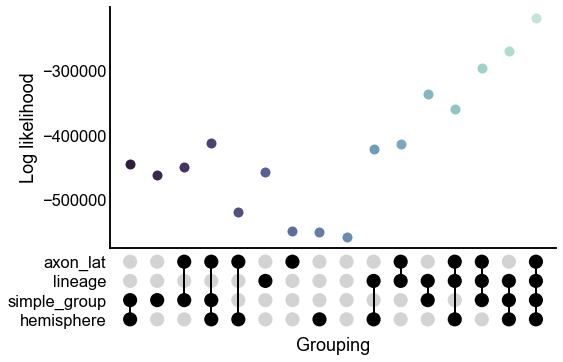
upset_stripplot(results, y="lik", ax=ax, **stripplot_kws)
ax.set(ylabel="Log likelihood")
stashfig("all-model-lik")
fig, ax = plt.subplots(1, 1, figsize=(8, 6))
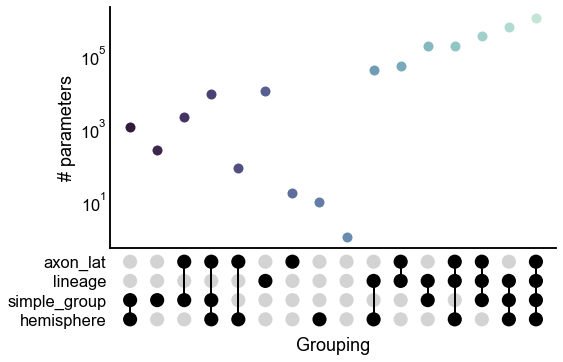
upset_stripplot(results, y="n_params", ax=ax, **stripplot_kws)
ax.set(ylabel="# parameters")
ax.set_yscale("log")
stashfig("all-model-n_params")
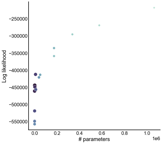
Look at the tradeoff between complexity and fit
fig, ax = plt.subplots(1, 1, figsize=(8, 8))
sns.scatterplot(
data=results,
x="n_params",
y="lik",
hue="group_keys",
palette=palette,
legend=False,
size="rank",
ax=ax,
)
ax.set(xlabel="# parameters", ylabel="Log likelihood")
stashfig("all-model-n_params-vs-lik")
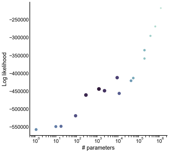
fig, ax = plt.subplots(1, 1, figsize=(8, 8))
sns.scatterplot(
data=results,
x="n_params",
y="lik",
hue="group_keys",
palette=palette,
legend=False,
size="rank",
ax=ax,
)
ax.set(xlabel="# parameters", ylabel="Log likelihood")
ax.set_xscale("log")
stashfig("all-model-n_params-vs-lik-logx")