Modularity
Modularity is a mathematical notion of how assortative a network is under some partition of the network into different groups (or communities, or modules, etc.). Here we apply a modularity maximization algorithm to the maggot network separated by edge types and compare various properties of the partitions and modularities.
Preliminaries
from pkg.utils import set_warnings

import datetime
import time

import matplotlib.pyplot as plt
import networkx as nx
import numpy as np
import pandas as pd
import seaborn as sns
from giskard.plot import crosstabplot
from graspologic.partition import leiden, modularity
from graspologic.utils import symmetrize
from pkg.data import load_maggot_graph, load_palette
from pkg.io import savefig
from pkg.plot import set_theme
from sklearn.metrics import adjusted_rand_score
from src.hierarchy import signal_flow
from src.visualization import adjplot

t0 = time.time()

set_theme()


def stashfig(name, **kwargs):
    foldername = "modularity"
    savefig(name, foldername=foldername, **kwargs)
Load the data
edge_types = [
    "ad",
    "aa",
    "dd",
    "da",
    "sum",
]
colors = sns.color_palette("deep", desat=None)
edge_type_palette = dict(zip(edge_types, colors))
nice_edge_types = dict(
    zip(edge_types, [r"A $\to$ D", r"A $\to$ A", r"D $\to$ D", r"D $\to$ A", "Sum"])
)
palette = load_palette()
mg = load_maggot_graph()
mg = mg[mg.nodes["paper_clustered_neurons"]]
mg.to_largest_connected_component()
adj = mg.sum.adj
sf = signal_flow(adj)
mg.nodes["neg_sf"] = -sf
mg.nodes["sf"] = sf
Optimize modularity
Here I use Leiden to find partitions which maximize the modularity score.
def preprocess_for_leiden(adj):
    sym_adj = adj.copy()
    sym_adj = symmetrize(sym_adj)

    # convert datatype
    # NOTE: have to do some weirdness because leiden only wants str keys right now
    undirected_g = nx.from_numpy_array(sym_adj)
    str_arange = [f"{i}" for i in range(len(undirected_g))]
    arange = np.arange(len(undirected_g))
    str_node_map = dict(zip(arange, str_arange))
    nx.relabel_nodes(undirected_g, str_node_map, copy=False)
    return undirected_g


def optimize_leiden(g, n_restarts=25, resolution=1, randomness=0.001):
    best_modularity = -np.inf
    best_partition = {}
    for i in range(n_restarts):
        partition = leiden(
            g,
            resolution=resolution,
            randomness=randomness,
            check_directed=False,
            extra_forced_iterations=10,
        )
        modularity_score = modularity(g, partitions=partition, resolution=resolution)
        if modularity_score > best_modularity:
            best_partition = partition
            best_modularity = modularity_score
    return best_partition, best_modularity


nodelist = mg.nodes.index
n_restarts = 50
randomness = 0.01
resolution = 1.0
rows = []
currtime = time.time()
for edge_type in edge_types:
    edge_type_mg = mg.to_edge_type_graph(edge_type)
    adj = edge_type_mg.adj
    sym_g = preprocess_for_leiden(adj)
    partition, modularity_score = optimize_leiden(
        sym_g,
        n_restarts=n_restarts,
        resolution=resolution,
        randomness=randomness,
    )
    str_arange = [f"{i}" for i in range(len(sym_g))]
    flat_partition = list(map(partition.get, str_arange))
    row = {
        "modularity_score": modularity_score,
        "resolution": resolution,
        "edge_type": edge_type,
        "nice_edge_type": nice_edge_types[edge_type],
        "partition": flat_partition,
        "adj": adj,
        "g": sym_g,
    }
    rows.append(row)

print(f"{time.time() - currtime:.3f} seconds elapsed to fit all partitions.")
results = pd.DataFrame(rows)
149.793 seconds elapsed to fit all partitions.
Plot results
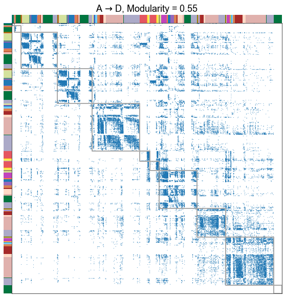
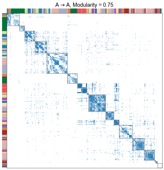
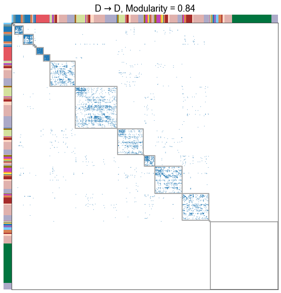
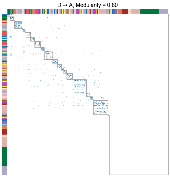
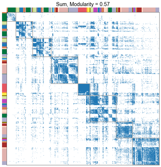
Plot the adjacency matrices sorted by fit partition
for _, row in results.iterrows():
    edge_type = row["edge_type"]
    nice_edge_type = nice_edge_types[edge_type]
    adj = row["adj"]
    meta = mg.nodes
    meta["partition"] = row["partition"]
    meta["partition"] = meta["partition"].fillna(-1)
    meta["is_unpartitioned"] = meta["partition"] == -1
    modularity_score = row["modularity_score"]
    adjplot(
        adj,
        meta=meta,
        sort_class="partition",
        class_order=["is_unpartitioned", "neg_sf"],
        colors="simple_group",
        palette=palette,
        plot_type="scattermap",
        item_order=["simple_group", "neg_sf"],
        ticks=False,
        sizes=(1, 2),
        gridline_kws=dict(linewidth=0),
        title=f"{nice_edge_type}, Modularity = {modularity_score:.2f}",
        blocklines="partition",
    )
    stashfig(f"modularity-sorted-adj-edge_type={edge_type}")
Plot the modularity for each edge type
fig, ax = plt.subplots(1, 1, figsize=(8, 6))
sns.stripplot(
    data=results, jitter=False, x="nice_edge_type", y="modularity_score", ax=ax
)
ax.set(ylabel="Modularity", xlabel="")
stashfig("modularity-by-edge-type")
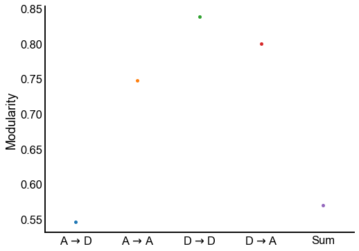
Conclusion
The different edge types have distinct modularities (we should be able to get p-values for this). In particular, the A to D seems the least modular.
Plot the similarities between modularity-maximizing partitions
def compute_pairwise_ari(results):
    pairwise = pd.DataFrame(index=results.index, columns=results.index, dtype=float)
    # pairwise.index.name = None
    # pairwise.columns.name = None
    for idx1, row1 in results.iterrows():
        for idx2, row2 in results.iterrows():
            partition1 = row1["partition"]
            partition2 = row2["partition"]
            partition1 = np.array(partition1)
            partition2 = np.array(partition2)
            partition1[partition1 == None] = -1
            partition2[partition2 == None] = -1
            isvalid1 = partition1 != -1
            isvalid2 = partition2 != -1
            keep_inds = np.where(isvalid1 & isvalid2)[0]
            ari = adjusted_rand_score(partition1[keep_inds], partition2[keep_inds])
            pairwise.loc[idx1, idx2] = ari
    return pairwise


pairwise_ari = compute_pairwise_ari(results.set_index("nice_edge_type"))

fig, ax = plt.subplots(1, 1, figsize=(6, 6))

inds = np.tril_indices(len(pairwise_ari), k=0)
mask = np.zeros((len(pairwise_ari), len(pairwise_ari)), dtype=bool)
mask[inds] = 1
sns.heatmap(
    pairwise_ari,
    ax=ax,
    square=True,
    annot=True,
    mask=mask,
    vmin=0,
    vmax=1,
    center=0,
    cmap="RdBu_r",
    cbar=False,
)
ax.set(xlabel="Edge type", ylabel="Edge type", title="Partition ARIs")
plt.setp(ax.get_yticklabels(), rotation=0)
stashfig("pairwise-aris-modularity")
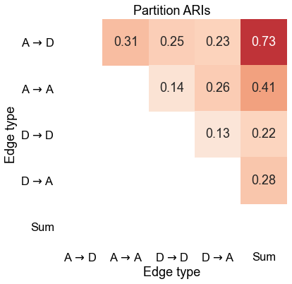
Conclusion
The modularity-maximizing partitions between the different edge types are quite different. Put another way, the “modules” you get by looking at each edge type separately don’t seem very similar.
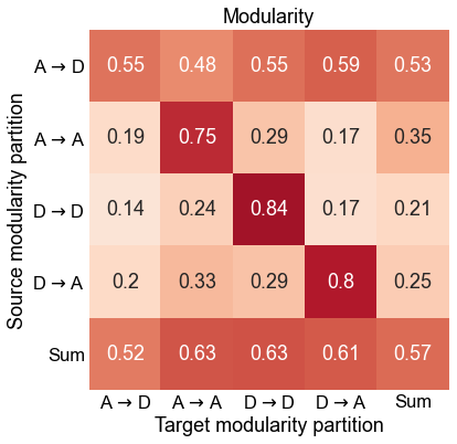
Plot the modularity of one edge type graph under another’s fit partition
edge_sorted_results = results.set_index("nice_edge_type")
pairwise_modularity = pd.DataFrame(
    index=edge_sorted_results.index, columns=edge_sorted_results.index, dtype=float
)
for idx1, row1 in edge_sorted_results.iterrows():
    for idx2, row2 in edge_sorted_results.iterrows():
        source_partition = row1["partition"]
        source_partition = [str(s) for s in source_partition]
        nodes = [str(s) for s in range(len(source_partition))]
        partition_map = dict(zip(nodes, source_partition))
        target_g = row2["g"]
        modularity_score = modularity(target_g, partition_map)
        pairwise_modularity.loc[idx1, idx2] = modularity_score
pairwise_modularity

fig, ax = plt.subplots(1, 1, figsize=(6, 6))
sns.heatmap(
    pairwise_modularity,
    ax=ax,
    square=True,
    annot=True,
    vmin=0,
    vmax=1,
    center=0,
    cmap="RdBu_r",
    cbar=False,
)
ax.set(
    xlabel="Target modularity partition",
    ylabel="Source modularity partition",
    title="Modularity",
)
plt.setp(ax.get_yticklabels(), rotation=0)
stashfig("pairwise-modularity")
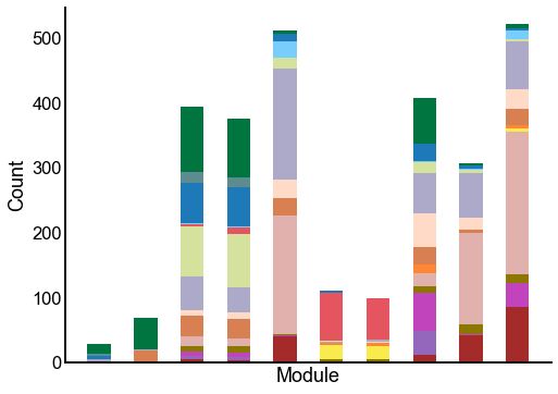
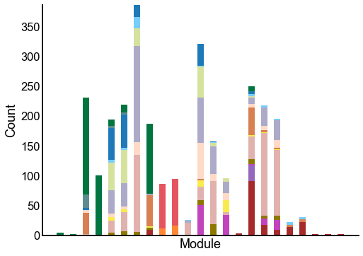
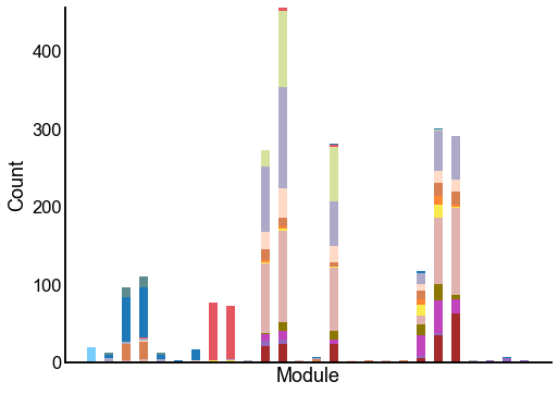
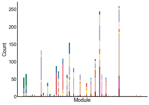
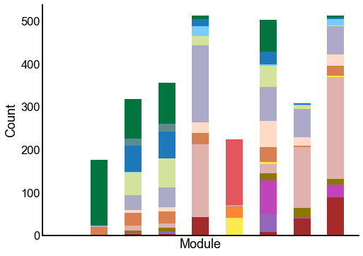
Plot the composition of the predicted modules
for _, row in results.iterrows():
    edge_type = row["edge_type"]
    nice_edge_type = nice_edge_types[edge_type]
    adj = row["adj"]
    meta = mg.nodes
    meta["partition"] = row["partition"]
    ax = crosstabplot(
        meta,
        group="partition",
        group_order="sf",
        hue="simple_group",
        hue_order="sf",
        palette=palette,
    )
    ax.set(xlabel="Module", xticks=[])
    stashfig(f"{edge_type}-crosstabplot")
End
elapsed = time.time() - t0
delta = datetime.timedelta(seconds=elapsed)
print("----")
print(f"Script took {delta}")
print(f"Completed at {datetime.datetime.now()}")
print("----")
----
Script took 0:03:36.493232
Completed at 2021-04-27 09:04:25.451133
----