.ipynb .pdf

repository open issue

Contents

Look at it

Preliminaries

from pkg.utils import set_warnings

import datetime
import time

import matplotlib.pyplot as plt
import numpy as np
import seaborn as sns
from graspologic.embed import selectSVD
from sklearn.preprocessing import normalize
from graspologic.utils import pass_to_ranks
from umap import AlignedUMAP
from giskard.plot import graphplot
from src.visualization import CLASS_COLOR_DICT

from graspologic.align import OrthogonalProcrustes, SeedlessProcrustes
from graspologic.embed import (
    AdjacencySpectralEmbed,
    OmnibusEmbed,
    select_dimension,
)
from graspologic.match import GraphMatch
from graspologic.plot import pairplot
from graspologic.utils import (
    augment_diagonal,
    binarize,
    multigraph_lcc_intersection,
    pass_to_ranks,
)
from pkg.data import (
    load_maggot_graph,
    load_palette,
    select_nice_nodes,
    load_node_palette,
    load_network_palette,
)
from pkg.io import savefig
from pkg.plot import set_theme
from giskard.utils import get_paired_inds

from src.visualization import adjplot  # TODO fix graspologic version and replace here
from giskard.plot import graphplot
from matplotlib.colors import LinearSegmentedColormap
from scipy.stats import binom


def stashfig(name, **kwargs):
    foldername = "look_at_it"
    savefig(name, foldername=foldername, **kwargs)

Load and process data

t0 = time.time()
set_theme()

network_palette, NETWORK_KEY = load_network_palette()
node_palette, NODE_KEY = load_node_palette()

mg = load_maggot_graph()
mg = select_nice_nodes(mg)
nodes = mg.nodes
left_nodes = nodes[nodes["hemisphere"] == "L"]
left_inds = left_nodes["_inds"]
right_nodes = nodes[nodes["hemisphere"] == "R"]
right_inds = right_nodes["_inds"]
left_paired_inds, right_paired_inds = get_paired_inds(
    nodes, pair_key="predicted_pair", pair_id_key="predicted_pair_id"
)
right_paired_inds_shifted = right_paired_inds - len(left_inds)
adj = mg.sum.adj
ll_adj = adj[np.ix_(left_inds, left_inds)]
rr_adj = adj[np.ix_(right_inds, right_inds)]

Removed 13 nodes when taking the largest connected component.
Removed 38 nodes when removing pendants.
Removed 0 nodes when taking the largest connected component.

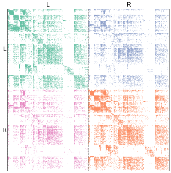
Plot the ipsilateral subgraph adjacency matrices

def calculate_weighted_degrees(adj):
    return np.sum(adj, axis=0) + np.sum(adj, axis=1)


color_matrix = np.zeros_like(adj)
color_matrix[np.ix_(left_inds, left_inds)] = 0
color_matrix[np.ix_(right_inds, right_inds)] = 1
color_matrix[np.ix_(left_inds, right_inds)] = 2
color_matrix[np.ix_(right_inds, left_inds)] = 3
edge_palette = dict(zip(np.arange(4), sns.color_palette("Set2")))
nodes["degree"] = -calculate_weighted_degrees(adj)
adjplot(
    adj,
    plot_type="scattermap",
    sizes=(1, 1),
    meta=nodes,
    sort_class=["hemisphere"],
    item_order=["simple_group", "degree"],
    tick_fontsize=20,
    color_matrix=color_matrix,
    edge_palette=edge_palette,
)

stashfig("adj-degree-sort")

Fit a 2-block model

n_left = len(left_inds)
n_right = len(right_inds)
# Note: graspologic has some code to do most of this but I wanted everything here to be
# above ground so to speak
# TODO ignore loops?
ll_n_edges = np.count_nonzero(adj[np.ix_(left_inds, left_inds)])
rr_n_edges = np.count_nonzero(adj[np.ix_(right_inds, right_inds)])
lr_n_edges = np.count_nonzero(adj[np.ix_(left_inds, right_inds)])
rl_n_edges = np.count_nonzero(adj[np.ix_(right_inds, left_inds)])
n_edges_matrix = np.array([[ll_n_edges, lr_n_edges], [rl_n_edges, rr_n_edges]])

ll_p_edge = ll_n_edges / (n_left ** 2)
rr_p_edge = rr_n_edges / (n_right ** 2)
lr_p_edge = lr_n_edges / (n_left * n_right)
rl_p_edge = rl_n_edges / (n_left * n_right)
p_edge_matrix = np.array([[ll_p_edge, lr_p_edge], [rl_p_edge, rr_p_edge]])

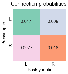
Plot the connection probability matrix

colors = sns.color_palette("Set2")


def make_custom_cmap(to_rgb, from_rgb=(1, 1, 1)):
    # REF: https://stackoverflow.com/questions/16267143/matplotlib-single-colored-colormap-with-saturation
    # from color r,g,b
    r1, g1, b1 = from_rgb

    # to color r,g,b
    r2, g2, b2 = to_rgb

    cdict = {
        "red": ((0, r1, r1), (1, r2, r2)),
        "green": ((0, g1, g1), (1, g2, g2)),
        "blue": ((0, b1, b1), (1, b2, b2)),
    }

    cmap = LinearSegmentedColormap("custom_cmap", cdict)
    return cmap


# forgive me god for what I'm about to do
fig, axs = plt.subplots(2, 2, figsize=(4, 4), gridspec_kw=dict(hspace=0, wspace=0))
heatmap_kws = dict(
    vmin=0, vmax=0.02, annot=True, cbar=False, xticklabels=False, yticklabels=False
)


def plot_heatmap_element(value, color, ax):
    cmap = make_custom_cmap(color)
    sns.heatmap(np.array([[value]]), cmap=cmap, ax=ax, **heatmap_kws)


values = [ll_p_edge, lr_p_edge, rl_p_edge, rr_p_edge]
ordered_colors = [colors[0], colors[2], colors[3], colors[1]]

for i, (val, col) in enumerate(zip(values, ordered_colors)):
    plot_heatmap_element(val, col, axs.flat[i])
axs[0, 0].set_ylabel("L", rotation=0, labelpad=10)
axs[1, 0].set_ylabel("R", rotation=0, labelpad=10)
axs[1, 0].set_xlabel("L")
axs[1, 1].set_xlabel("R")
fig.suptitle("Connection probabilities")
fig.text(0, 0.385, "Presynaptic", ha="center", rotation=90)
fig.text(0.52, -0.02, "Postsynaptic", ha="center")
stashfig("connection-probabilities")

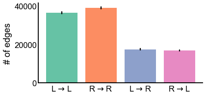
Plot the number of edges for each lateral type with 99% confidence intervals

fig, ax = plt.subplots(1, 1, figsize=(6, 3))
ns = [n_left ** 2, n_right ** 2, n_left * n_right, n_left * n_right]
edge_counts = [ll_n_edges, rr_n_edges, lr_n_edges, rl_n_edges]
for i, (n_edges, n) in enumerate(zip(edge_counts, ns)):
    p_edge = n_edges / n
    err = binom(n, p_edge).interval(0.99)
    err = np.array(err)
    ax.bar(i, n_edges, color=colors[i])
    ax.plot([i, i], err, color="black", zorder=90)
names = [r"L $\to$ L", r"R $\to$ R", r"L $\to$ R", r"R $\to$ L"]
ax.xaxis.set_major_locator(plt.FixedLocator(np.arange(4)))
ax.set(ylabel="# of edges", xticklabels=names)
stashfig("n_edges_plot")

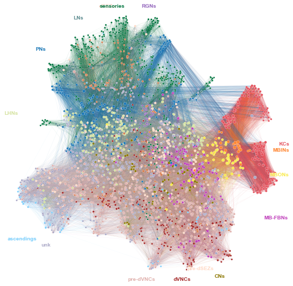
Plot a network layout of the whole network

ax = graphplot(
    network=adj,
    meta=nodes,
    n_components=64,
    n_neighbors=64,
    min_dist=0.8,
    hue=NODE_KEY,
    node_palette=node_palette,
    random_state=888888,
    sizes=(10, 40),
    hue_labels="radial",
    hue_label_fontsize="xx-small",
    adjust_labels=True,
    # verbose=True,
)
stashfig("whole-network-layout")

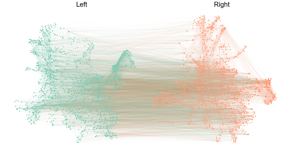
Plot the network split out by left/right

side_palette = dict(zip(["L", "R"], sns.color_palette("Set2")))
# edge_palette = dict(
#     zip([("L", "L"), ("R", "R"), ("L", "R"), ("R", "L")], sns.color_palette("Set2"))
# )
ax = graphplot(
    network=adj,
    meta=nodes,
    n_components=64,
    n_neighbors=64,
    min_dist=0.8,
    hue="hemisphere",
    node_palette=side_palette,
    random_state=888888,
    sizes=(10, 40),
    hue_label_fontsize="xx-small",
    tile="hemisphere",
    tile_layout=[["L", "R"]],
    figsize=(20, 10),
    edge_linewidth=0.2,
    edge_alpha=0.2,
    subsample_edges=0.2,
    # edge_hue="prepost",
    # edge_palette=edge_palette,
    # hue_labels="radial",
    # adjust_labels=True,
    # verbose=True,
)
ax.text(0, 1, "Left", fontsize="x-large")
ax.text(2, 1, "Right", fontsize="x-large")
stashfig("split-network-layout")

Simple statistics for the left hemisphere induced subgraph

ll_mg, rr_mg, _, _ = mg.bisect(paired=False)
ll_mg.sum

	n_nodes	n_edges	sum_edge_weights
edge_type
sum	1481.0	36447.0	117068.0

Simple statistics for the right hemisphere induced subgraph

rr_mg.sum

	n_nodes	n_edges	sum_edge_weights
edge_type
sum	1481.0	39096.0	129527.0

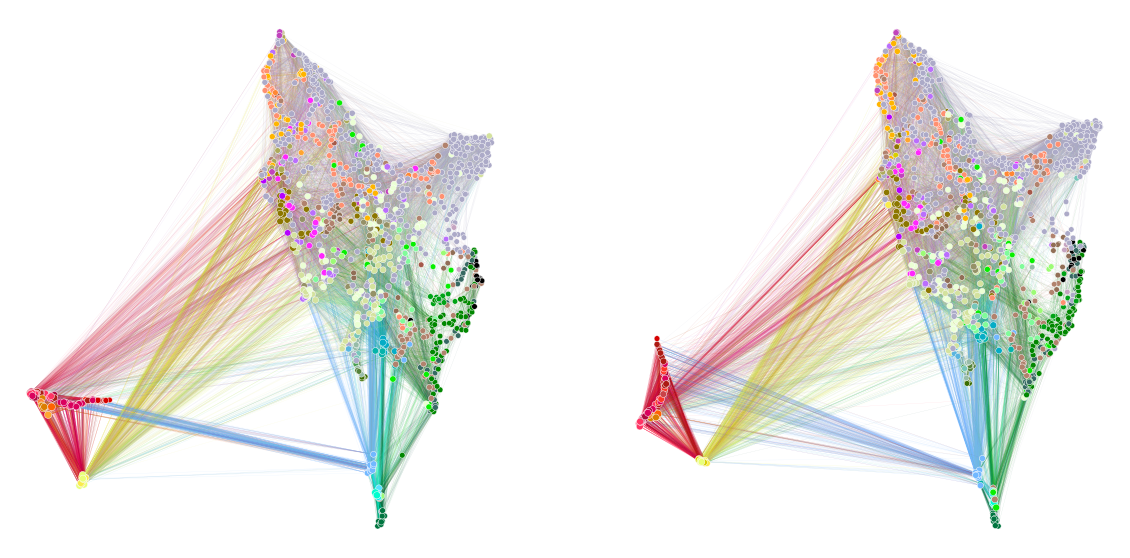
[Experimental] Plot a graph layout for each hemisphere using aligned UMAP

def ase(adj, n_components=None):
    U, S, Vt = selectSVD(adj, n_components=n_components, algorithm="full")
    S_sqrt = np.diag(np.sqrt(S))
    X = U @ S_sqrt
    Y = Vt.T @ S_sqrt
    return X, Y


def prescale_for_embed(adjs):
    norms = [np.linalg.norm(adj, ord="fro") for adj in adjs]
    mean_norm = np.mean(norms)
    adjs = [adjs[i] * mean_norm / norms[i] for i in range(len(adjs))]
    return adjs


n_components = 16  # 24 looked fine
power = True
normed = False
if power:
    ll_adj_for_umap = pass_to_ranks(ll_adj)
    rr_adj_for_umap = pass_to_ranks(rr_adj)
    if normed:
        ll_adj_for_umap = normalize(ll_adj_for_umap, axis=1)
        rr_adj_for_umap = normalize(rr_adj_for_umap, axis=1)
    ll_adj_for_umap = ll_adj_for_umap @ ll_adj_for_umap
    rr_adj_for_umap = rr_adj_for_umap @ rr_adj_for_umap
else:
    ll_adj_for_umap = pass_to_ranks(ll_adj)
    rr_adj_for_umap = pass_to_ranks(rr_adj)

X_ll, Y_ll = ase(ll_adj_for_umap, n_components=n_components)
X_rr, Y_rr = ase(rr_adj_for_umap, n_components=n_components)

Z_ll = np.concatenate((X_ll, Y_ll), axis=1)
Z_rr = np.concatenate((X_rr, Y_rr), axis=1)
# Z_ll, _ = ase(Z_ll, n_components=n_components)
# Z_rr, _ = ase(Z_rr, n_components=n_components)

relation_dict = dict(zip(left_paired_inds, right_paired_inds_shifted))

aumap = AlignedUMAP(
    random_state=88888,
    n_neighbors=32,
    min_dist=0.95,
    metric="cosine",
    alignment_regularisation=1e-2,
)
umap_embeds = aumap.fit_transform([Z_ll, Z_rr], relations=[relation_dict])

graphplot_kws = dict(sizes=(30, 60))
fig, axs = plt.subplots(1, 2, figsize=(20, 10))
graphplot(
    network=ll_adj,
    embedding=umap_embeds[0],
    meta=left_nodes,
    hue="merge_class",
    node_palette=CLASS_COLOR_DICT,
    ax=axs[0],
    **graphplot_kws,
)
graphplot(
    network=rr_adj,
    embedding=umap_embeds[1],
    meta=right_nodes,
    hue="merge_class",
    node_palette=CLASS_COLOR_DICT,
    ax=axs[1],
    **graphplot_kws,
)
stashfig("aligned-umap-layout")

elapsed = time.time() - t0
delta = datetime.timedelta(seconds=elapsed)
print("----")
print(f"Script took {delta}")
print(f"Completed at {datetime.datetime.now()}")
print("----")

----
Script took 0:02:39.102026
Completed at 2021-05-12 18:58:23.461493
----

Introduction Look at RDPG models