Testing bilateral symmetry
This notebook describes a first pass at testing for some notion of bilateral symmetry. Here, we focus only on the left-left and right-right induced subgraphs for simplicity. We also use the unweighted version of the maggot connectomes. Also, for now, we restrict ourselves to the set of neurons for which we know a pairing between neuron A on the left hemisphere and neuron A on the right hemisphere.
To summarize, this notebook presents a strange phenomena where depending on the dimension of the embedding that we use to test bilateral symmetry, we get vastly different results.
We also present a modified proceedure that fails to reject the null that the latent positions of the left-left induced subgraph and the right-right induced subgraph have the same distribution over many embedding dimensions, suggesting that for the current setup we fail to reject bilateral symmetry.
Preliminaries
from pkg.utils import set_warnings

set_warnings()

import datetime
import pprint
import time


import matplotlib.pyplot as plt
import numpy as np
import pandas as pd
import seaborn as sns
from hyppo.ksample import KSample
from scipy.stats import epps_singleton_2samp, ks_2samp


from graspologic.align import OrthogonalProcrustes, SeedlessProcrustes
from graspologic.embed import AdjacencySpectralEmbed, select_dimension
from graspologic.plot import pairplot
from graspologic.utils import (
    augment_diagonal,
    binarize,
    multigraph_lcc_intersection,
    pass_to_ranks,
)
from pkg.data import load_adjacency, load_node_meta
from pkg.io import savefig
from pkg.plot import set_theme
from pkg.utils import get_paired_inds, get_paired_subgraphs

from src.visualization import adjplot  # TODO fix graspologic version and replace here

t0 = time.time()


def stashfig(name, **kwargs):
    foldername = "bilateral_symmetry"
    savefig(name, foldername=foldername, **kwargs)


colors = sns.color_palette("Set1")
palette = dict(zip(["Left", "Right", "OP", "O-SP"], colors))
set_theme()
/Users/bpedigo/miniconda3/envs/maggot-revamp/lib/python3.8/site-packages/umap/__init__.py:9: UserWarning: Tensorflow not installed; ParametricUMAP will be unavailable
  warn("Tensorflow not installed; ParametricUMAP will be unavailable")
Load the data
Load node metadata and select the subgraphs of interest
meta = load_node_meta()
meta = meta[meta["paper_clustered_neurons"]]

adj = load_adjacency(graph_type="G", nodelist=meta.index)

lp_inds, rp_inds = get_paired_inds(meta)
left_meta = meta.iloc[lp_inds]
right_meta = meta.iloc[rp_inds]

ll_adj, rr_adj, lr_adj, rl_adj = get_paired_subgraphs(adj, lp_inds, rp_inds)

# TODO not sure what we wanna do about LCCs here
adjs, lcc_inds = multigraph_lcc_intersection([ll_adj, rr_adj], return_inds=True)
ll_adj = adjs[0]
rr_adj = adjs[1]
print(f"{len(lcc_inds)} in intersection of largest connected components.")

print(f"Original number of valid pairs: {len(lp_inds)}")

left_meta = left_meta.iloc[lcc_inds]
right_meta = right_meta.iloc[lcc_inds]
meta = pd.concat((left_meta, right_meta))
n_pairs = len(ll_adj)

print(f"Number of pairs after taking LCC intersection: {n_pairs}")
1148 in intersection of largest connected components.
Original number of valid pairs: 1149
Number of pairs after taking LCC intersection: 1148
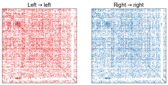
Plotting the aligned adjacency matrices
At a high level, we see that the left-left and right-right induced subgraphs look quite similar when aligned by the known neuron pairs.
fig, axs = plt.subplots(1, 2, figsize=(10, 5))
adjplot(
    ll_adj,
    plot_type="scattermap",
    sizes=(1, 2),
    ax=axs[0],
    title=r"Left $\to$ left",
    color=palette["Left"],
)
adjplot(
    rr_adj,
    plot_type="scattermap",
    sizes=(1, 2),
    ax=axs[1],
    title=r"Right $\to$ right",
    color=palette["Right"],
)
stashfig("left-right-induced-adjs")
Embedding the graphs
Here I embed the unweighted, directed graphs using ASE.
def plot_latents(left, right, title="", n_show=4):
    plot_data = np.concatenate([left, right], axis=0)
    labels = np.array(["Left"] * len(left) + ["Right"] * len(right))
    pg = pairplot(plot_data[:, :n_show], labels=labels, title=title)
    return pg


def screeplot(sing_vals, elbow_inds, color=None, ax=None, label=None):
    if ax is None:
        _, ax = plt.subplots(1, 1, figsize=(8, 4))
    plt.plot(range(1, len(sing_vals) + 1), sing_vals, color=color, label=label)
    plt.scatter(
        elbow_inds, sing_vals[elbow_inds - 1], marker="x", s=50, zorder=10, color=color
    )
    ax.set(ylabel="Singular value", xlabel="Index")
    return ax


def embed(adj, n_components=40, ptr=False):
    if ptr:
        adj = pass_to_ranks(adj)
    elbow_inds, elbow_vals = select_dimension(augment_diagonal(adj), n_elbows=4)
    elbow_inds = np.array(elbow_inds)
    ase = AdjacencySpectralEmbed(n_components=n_components)
    out_latent, in_latent = ase.fit_transform(adj)
    return out_latent, in_latent, ase.singular_values_, elbow_inds
Run the embedding
n_components = 8
max_n_components = 40
preprocess = "binarize"

if preprocess == "binarize":
    ll_adj = binarize(ll_adj)
    rr_adj = binarize(rr_adj)

left_out_latent, left_in_latent, left_sing_vals, left_elbow_inds = embed(
    ll_adj, n_components=max_n_components
)
right_out_latent, right_in_latent, right_sing_vals, right_elbow_inds = embed(
    rr_adj, n_components=max_n_components
)
Plot the screeplots
fig, ax = plt.subplots(1, 1, figsize=(8, 4))
screeplot(left_sing_vals, left_elbow_inds, color=palette["Left"], ax=ax, label="Left")
screeplot(
    right_sing_vals, right_elbow_inds, color=palette["Right"], ax=ax, label="Right"
)
ax.legend()
ax.axvline(n_components, color="black", linewidth=1.5, linestyle="--")
stashfig(f"screeplot-preprocess={preprocess}")
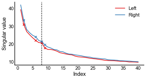
Calculating the Frobenius norm of the adjacency matrices
Note that in the screeplot above, the singular values of the right-right subgraph are always above those of the left-left subgraph (at least for this range of \(d\)). This hints as the “scale” of the two graphs. We’ve noticed that the left-left subgraph is slightly less dense than the right-right.
It is perhaps worth investigating whether to use the “scaled” version of the hypothesis test.
print(f"Norm of left-left adjacency: {np.linalg.norm(binarize(ll_adj))}")
print(f"Norm of right-right adjacency: {np.linalg.norm(binarize(rr_adj))}")
Norm of left-left adjacency: 163.6459593146131
Norm of right-right adjacency: 170.35551062410633
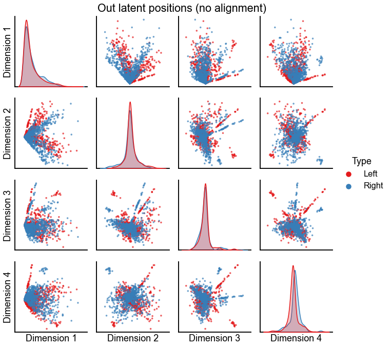
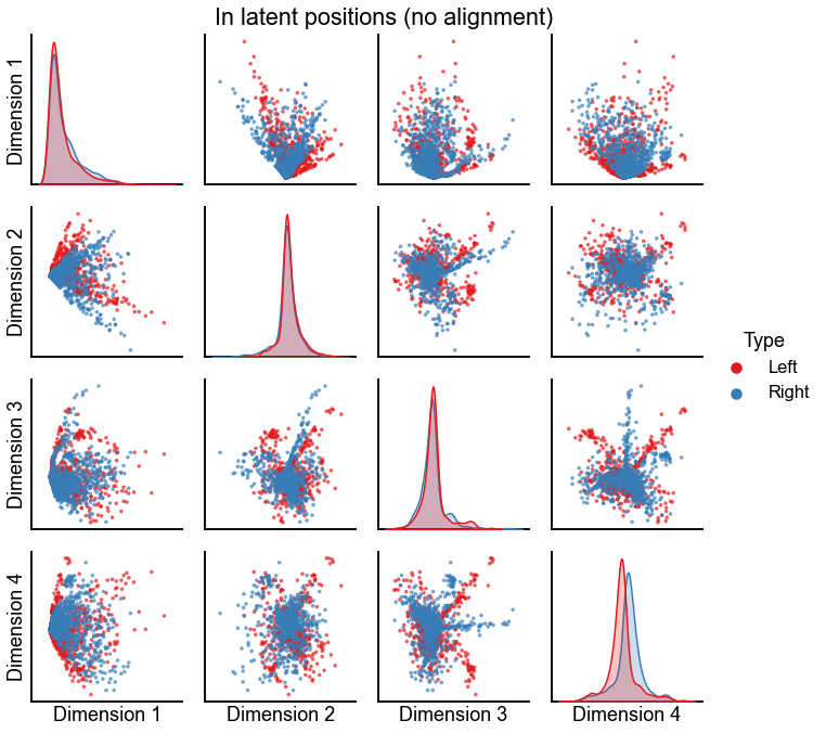
Plot the latent positions of both graphs before alignment
plot_latents(
    left_out_latent, right_out_latent, title="Out latent positions (no alignment)"
)
stashfig(f"out-latent-no-align-preprocess={preprocess}")
plot_latents(
    left_in_latent, right_in_latent, title="In latent positions (no alignment)"
)
stashfig(f"in-latent-no-align-preprocess={preprocess}")
Align the embeddings
Here we align first using orthogonal Procrustes (OP), and then using seedless Procrustes initialized at the orthogonal Procrustes solution (O-SP).
I also calculate the Frobenius norm of the difference in the embeddings after performing the alignment.
def run_alignments(X, Y, scale=False):
    X = X.copy()
    Y = Y.copy()
    if scale:
        X_norm = np.linalg.norm(X, ord="fro")
        Y_norm = np.linalg.norm(Y, ord="fro")
        avg_norms = (X_norm + Y_norm) / 2
        X = X * (avg_norms / X_norm)
        Y = Y * (avg_norms / Y_norm)
    op = OrthogonalProcrustes()
    X_trans_op = op.fit_transform(X, Y)
    sp = SeedlessProcrustes(init="custom", initial_Q=op.Q_)
    X_trans_sp = sp.fit_transform(X, Y)
    return X_trans_op, X_trans_sp


def calc_diff_norm(X, Y):
    return np.linalg.norm(X - Y, ord="fro")
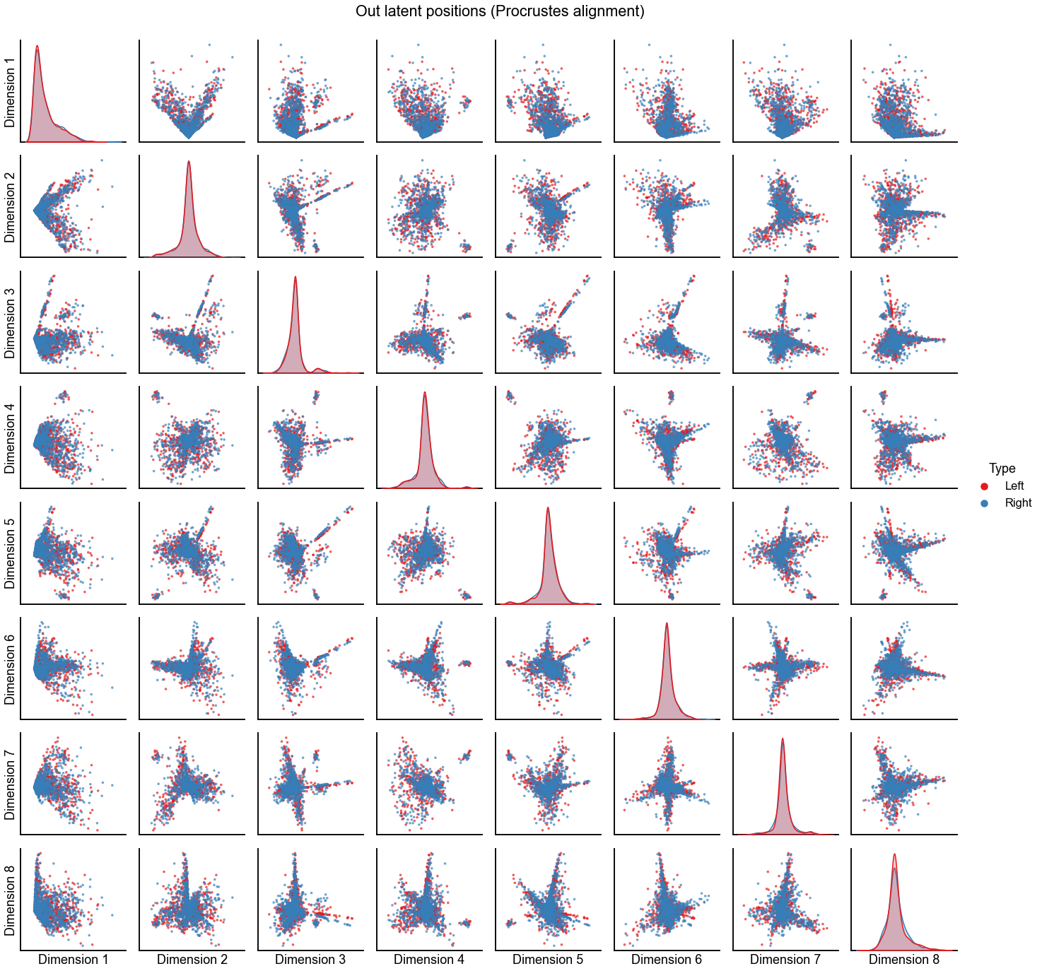
Plot the alignment for d=8 dimensions
n_components = 8
op_left_out_latent, sp_left_out_latent = run_alignments(
left_out_latent[:, :n_components], right_out_latent[:, :n_components]
)
op_diff_norm = calc_diff_norm(op_left_out_latent, right_out_latent[:, :n_components])
sp_diff_norm = calc_diff_norm(sp_left_out_latent, right_out_latent[:, :n_components])
print(f"Procrustes diff. norm using true pairs: {op_diff_norm:0.3f}")
print(f"Seedless Procrustes diff. norm using true pairs: {sp_diff_norm:0.3f}")
plot_latents(
op_left_out_latent,
right_out_latent[:, :n_components],
"Out latent positions (Procrustes alignment)",
n_show=n_components,
)
stashfig(f"out-latent-op-preprocess={preprocess}")
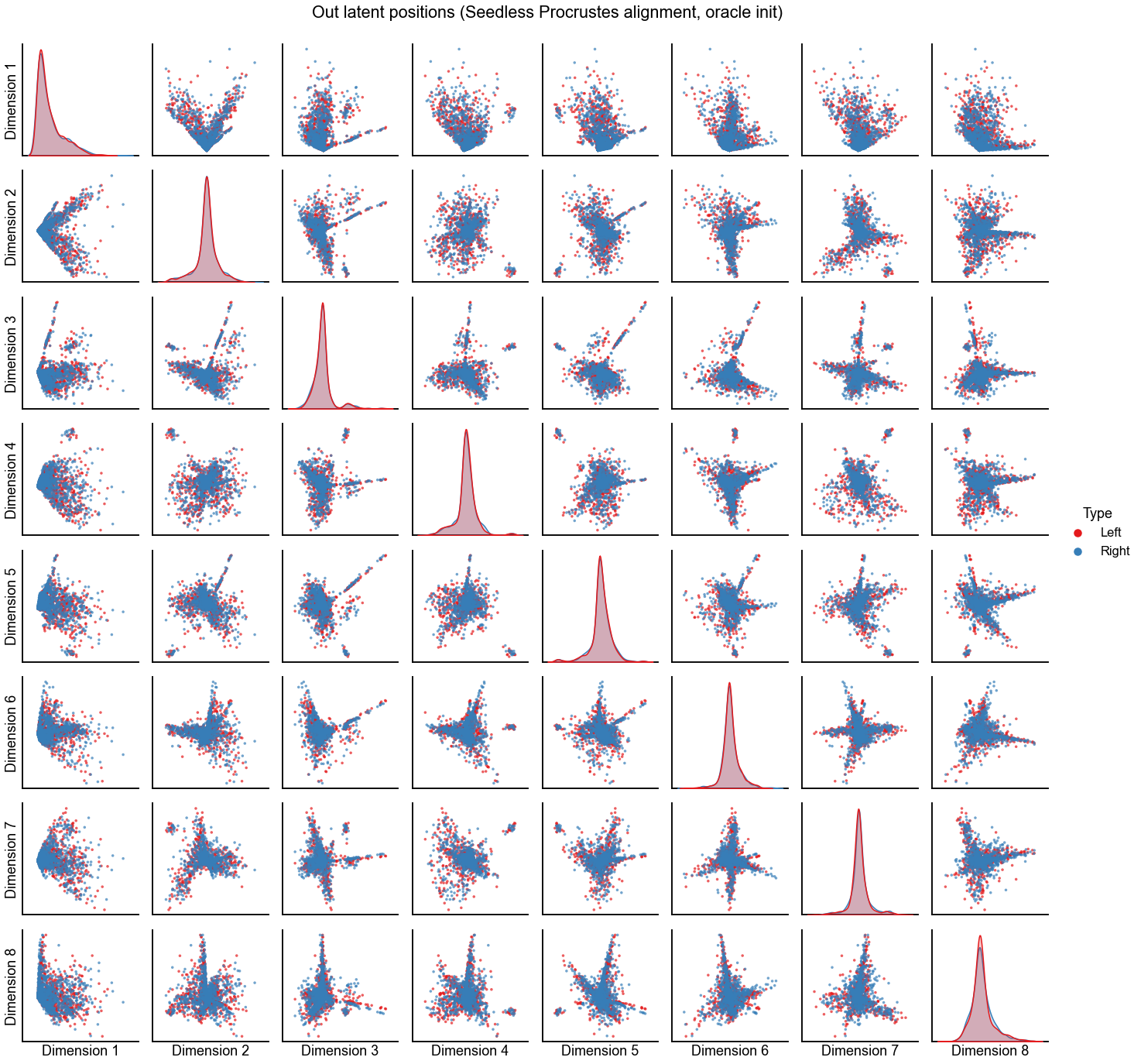
plot_latents(
sp_left_out_latent,
right_out_latent[:, :n_components],
"Out latent positions (Seedless Procrustes alignment, oracle init)",
n_show=n_components,
)
stashfig(f"out-latent-o-sp-n_components={n_components}-preprocess={preprocess}")
Procrustes diff. norm using true pairs: 4.732
Seedless Procrustes diff. norm using true pairs: 4.789
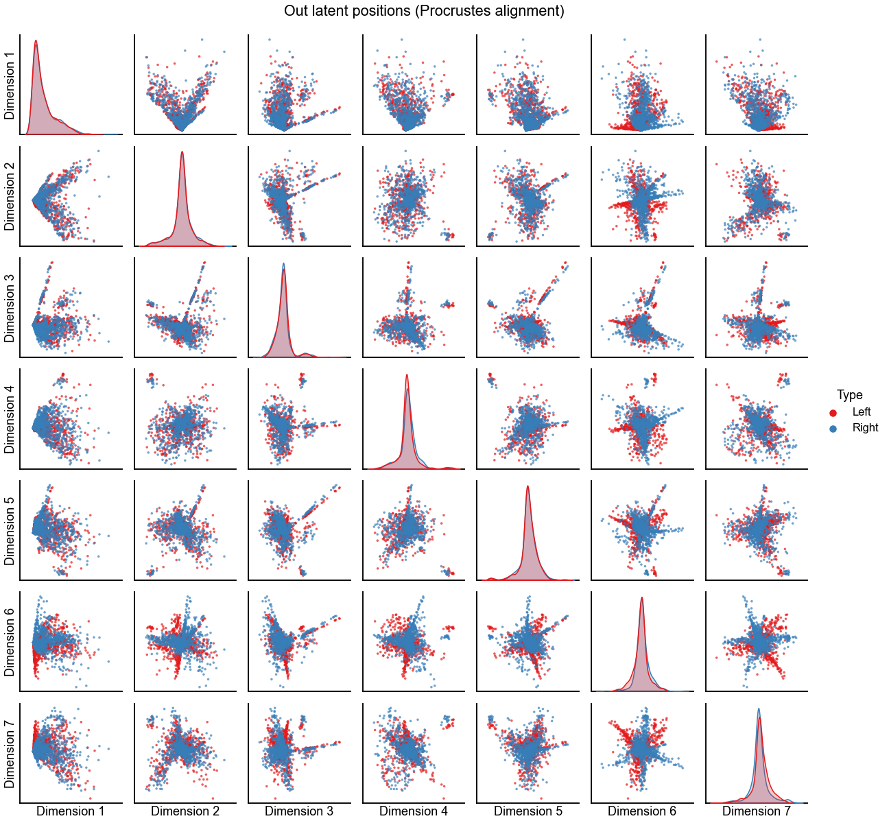
Plot the alignment for d=7 dimensions
n_components = 7
op_left_out_latent, sp_left_out_latent = run_alignments(
left_out_latent[:, :n_components], right_out_latent[:, :n_components]
)
op_diff_norm = calc_diff_norm(op_left_out_latent, right_out_latent[:, :n_components])
sp_diff_norm = calc_diff_norm(sp_left_out_latent, right_out_latent[:, :n_components])
print(f"Procrustes diff. norm using true pairs: {op_diff_norm:0.3f}")
print(f"Seedless Procrustes diff. norm using true pairs: {sp_diff_norm:0.3f}")
plot_latents(
op_left_out_latent,
right_out_latent[:, :n_components],
"Out latent positions (Procrustes alignment)",
n_show=n_components,
)
stashfig(f"out-latent-op-preprocess={preprocess}")
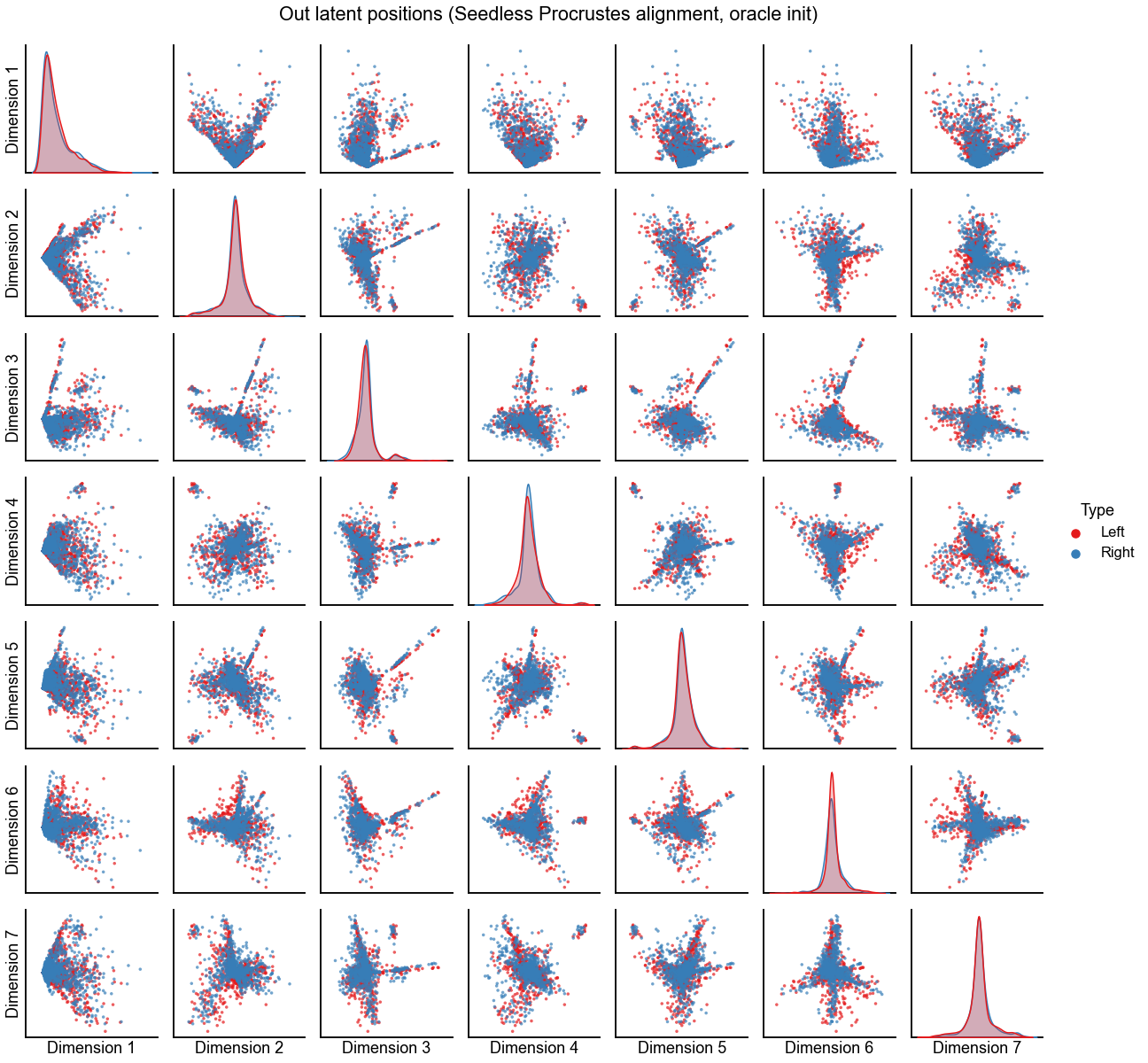
plot_latents(
sp_left_out_latent,
right_out_latent[:, :n_components],
"Out latent positions (Seedless Procrustes alignment, oracle init)",
n_show=n_components,
)
stashfig(f"out-latent-o-sp-n_components={n_components}-preprocess={preprocess}")
Procrustes diff. norm using true pairs: 7.238
Seedless Procrustes diff. norm using true pairs: 9.052
Hypothesis testing on the embeddings
To test whether the distribution of latent positions is different, we use the approach of the “nonpar” test, also called the latent distribution test. Here, for the backend 2-sample test, we use distance correlation (Dcorr).
test = "dcorr"
workers = -1
auto = True
if auto:
    n_bootstraps = None
else:
    n_bootstraps = 500


def run_test(
    X1,
    X2,
    rows=None,
    info={},
    auto=auto,
    n_bootstraps=n_bootstraps,
    workers=workers,
    test=test,
    print_out=False,
):
    currtime = time.time()
    test_obj = KSample(test)
    tstat, pvalue = test_obj.test(
        X1,
        X2,
        reps=n_bootstraps,
        workers=workers,
        auto=auto,
    )
    elapsed = time.time() - currtime
    row = {
        "pvalue": pvalue,
        "tstat": tstat,
        "elapsed": elapsed,
    }
    row.update(info)
    if print_out:
        pprint.pprint(row)
    if rows is not None:
        rows.append(row)
    else:
        return row
Run the two-sample test for varying embedding dimension
rows = []
for n_components in np.arange(1, 21):
    op_left_out_latent, sp_left_out_latent = run_alignments(
        left_out_latent[:, :n_components], right_out_latent[:, :n_components]
    )
    op_left_in_latent, sp_left_in_latent = run_alignments(
        left_in_latent[:, :n_components], right_in_latent[:, :n_components]
    )
    op_left_composite_latent = np.concatenate(
        (op_left_out_latent, op_left_in_latent), axis=1
    )
    sp_left_composite_latent = np.concatenate(
        (sp_left_out_latent, sp_left_in_latent), axis=1
    )
    right_composite_latent = np.concatenate(
        (right_out_latent[:, :n_components], right_in_latent[:, :n_components]), axis=1
    )

    run_test(
        op_left_composite_latent,
        right_composite_latent,
        rows,
        info={"alignment": "OP", "n_components": n_components},
    )
    run_test(
        sp_left_composite_latent,
        right_composite_latent,
        rows,
        info={"alignment": "O-SP", "n_components": n_components},
    )

results = pd.DataFrame(rows)
Plot the 2-sample test p-values by varying dimension
Note: these are on a log y-scale.
def plot_pvalues(results, line_locs=[0.05, 0.005, 0.0005]):
    results = results.copy()
    # jitter so we can see op vs o-sp
    op_results = results[results["alignment"] == "OP"]
    sp_results = results[results["alignment"] == "O-SP"]
    results.loc[op_results.index, "n_components"] += -0.15
    results.loc[sp_results.index, "n_components"] += 0.15

    styles = ["-", "--", ":"]
    line_kws = dict(color="black", alpha=0.7, linewidth=1.5, zorder=-1)

    # plot p-values by embedding dimension
    fig, ax = plt.subplots(1, 1, figsize=(10, 6))
    sns.scatterplot(
        data=results,
        x="n_components",
        y="pvalue",
        hue="alignment",
        palette=palette,
        ax=ax,
        s=40,
    )
    ax.set_yscale("log")
    styles = ["-", "--", ":"]
    line_kws = dict(color="black", alpha=0.7, linewidth=1.5, zorder=-1)
    for loc, style in zip(line_locs, styles):
        ax.axhline(loc, linestyle=style, **line_kws)
        ax.text(ax.get_xlim()[-1] + 0.1, loc, loc, ha="left", va="center")
    ax.set(xlabel="Dimension", ylabel="p-value")
    ax.get_legend().remove()
    ax.legend(bbox_to_anchor=(1.15, 1), loc="upper left", title="Alignment")

    xlim = ax.get_xlim()
    for x in range(1, int(xlim[1]), 2):
        ax.axvspan(x - 0.5, x + 0.5, color="lightgrey", alpha=0.2, linewidth=0)

    plt.tight_layout()


plot_pvalues(results)
stashfig(
    f"naive-pvalues-test={test}-n_bootstraps={n_bootstraps}-preprocess={preprocess}"
)
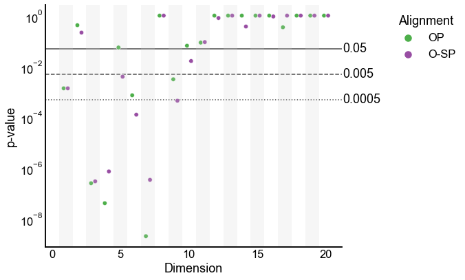
Not what we expected
It is worrisome that the p-values change drastically when the embedding dimension changes slightly.
Below, we investigate what could be causing this phenomenon.
Focus on the d=1 case
Note that in the testing above, even for \(d=1\), the latent positions were significantly different. Is this a bug? Or how can we explain this?
Set up some metadata for this experiment
left_arange = np.arange(n_pairs)
right_arange = left_arange + n_pairs
embedding_1d_df = pd.DataFrame(index=np.arange(2 * n_pairs))
embedding_1d_df["pair_ind"] = np.concatenate((left_arange, left_arange))
embedding_1d_df["hemisphere"] = "Right"
embedding_1d_df.loc[left_arange, "hemisphere"] = "Left"
embedding_1d_df["x"] = 1
embedding_1d_df.loc[left_arange, "x"] = 0
Align and test the d=1, out embedding
Just like in the 2-sample testing above, we take the \(d=1\) embedding, align the left to the right, and ask whether these embeddings are different. Here I only use the out latent positions.
n_components = 1
op_left_out_latent, sp_left_out_latent = run_alignments(
    left_out_latent[:, :n_components], right_out_latent[:, :n_components]
)
embedding_1d_df.loc[left_arange, "out_1d_align"] = op_left_out_latent[:, 0]
embedding_1d_df.loc[right_arange, "out_1d_align"] = right_out_latent[:, 0]

dcorr_results_1d_align = run_test(op_left_out_latent[:, :1], right_out_latent[:, :1])
ks_results_1d_align = ks_2samp(op_left_out_latent[:, 0], right_out_latent[:, 0])

print("DCorr 2-sample test on first out dimension, aligned in 1D:")
print(f"p-value = {dcorr_results_1d_align['pvalue']:0.4f}")

print("KS 2-sample test on first out dimension, aligned in 1D:")
print(f"p-value = {ks_results_1d_align[1]:0.4f}")
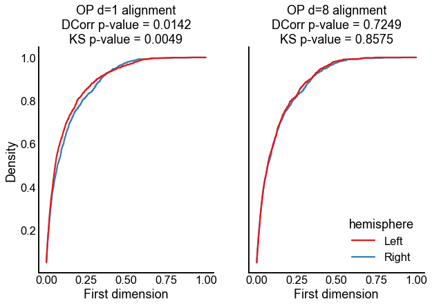
DCorr 2-sample test on first out dimension, aligned in 1D:
p-value = 0.0142
KS 2-sample test on first out dimension, aligned in 1D:
p-value = 0.0049
Align the \(d=8\) out embedding, test on the first dimension
Now, we instead perform the alignment in the \(d=8\) embedding. Then, we again look at only the first dimension of that aligned set of embeddings and test whether those are different.
n_components = 8
op_left_out_latent, sp_left_out_latent = run_alignments(
    left_out_latent[:, :n_components], right_out_latent[:, :n_components]
)

embedding_1d_df.loc[left_arange, "out_8d_align"] = op_left_out_latent[:, 0]
embedding_1d_df.loc[right_arange, "out_8d_align"] = right_out_latent[:, 0]

dcorr_results_8d_align = run_test(op_left_out_latent[:, :1], right_out_latent[:, :1])

ks_results_8d_align = ks_2samp(op_left_out_latent[:, 0], right_out_latent[:, 0])

print("DCorr 2-sample test on first out dimension, aligned in 8D:")
print(f"p-value = {dcorr_results_8d_align['pvalue']:0.4f}")

print("KS 2-sample test on first out dimension, aligned in 8D:")
print(f"p-value = {ks_results_8d_align[1]:0.4f}")
DCorr 2-sample test on first out dimension, aligned in 8D:
p-value = 0.7249
KS 2-sample test on first out dimension, aligned in 8D:
p-value = 0.8575
Plot the results for testing on the first dimension only
Below are empirical CDFs for the first dimension, in both of the cases described above. Note that in either case, the right embedding (blue line) is the same, because we aligned left to right.
fig, axs = plt.subplots(1, 2, figsize=(10, 6), sharey=True)
histplot_kws = dict(
    stat="density",
    cumulative=True,
    element="poly",
    common_norm=False,
    bins=np.linspace(0, 1, 2000),
    fill=False,
)

ax = axs[0]
sns.histplot(
    data=embedding_1d_df,
    x="out_1d_align",
    ax=ax,
    hue="hemisphere",
    legend=False,
    palette=palette,
    **histplot_kws,
)
title = "OP d=1 alignment"
title += f"\nDCorr p-value = {dcorr_results_1d_align['pvalue']:0.4f}"
title += f"\nKS p-value = {ks_results_1d_align[1]:0.4f}"
ax.set(title=title, xlabel="First dimension")

ax = axs[1]
sns.histplot(
    data=embedding_1d_df,
    x="out_8d_align",
    ax=ax,
    hue="hemisphere",
    palette=palette,
    **histplot_kws,
)
title = "OP d=8 alignment"
title += f"\nDCorr p-value = {dcorr_results_8d_align['pvalue']:0.4f}"
title += f"\nKS p-value = {ks_results_8d_align[1]:0.4f}"
ax.set(title=title, xlabel="First dimension")
stashfig(
    f"dim1-focus-cdf-test={test}-n_bootstraps={n_bootstraps}-preprocess={preprocess}"
)
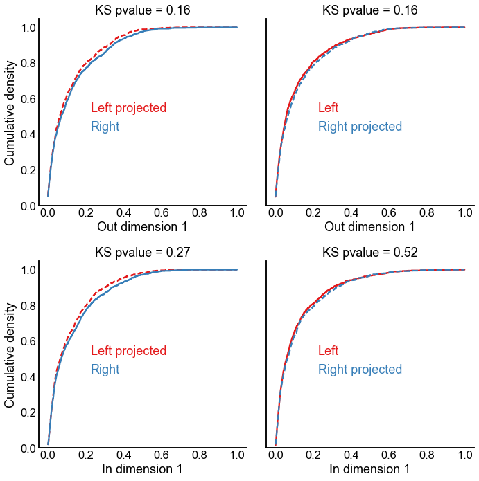
A projection experiment
Just to further put this issue of the first dimension to rest - here we look at what happens if we use the latent positions learned from the left to project the right-to-right adjacency matrix into the left latent space, and vice versa.
def get_projection_vector(v):
    v = v.copy()
    v /= np.linalg.norm(v) ** 2
    return v


y_l = get_projection_vector(left_in_latent[:, 0])
y_r = get_projection_vector(right_in_latent[:, 0])
x_l = get_projection_vector(left_out_latent[:, 0])
x_r = get_projection_vector(right_out_latent[:, 0])

embedding_1d_df.loc[right_arange, "out_1d_proj"] = rr_adj @ y_l
embedding_1d_df.loc[left_arange, "out_1d_proj"] = ll_adj @ y_r
embedding_1d_df.loc[right_arange, "in_1d_proj"] = rr_adj.T @ x_l
embedding_1d_df.loc[left_arange, "in_1d_proj"] = ll_adj.T @ x_r

embedding_1d_df.loc[right_arange, "out_1d_proj_unscale"] = embedding_1d_df.loc[
    right_arange, "out_1d_proj"
] / np.linalg.norm(embedding_1d_df.loc[right_arange, "out_1d_proj"])

embedding_1d_df.loc[left_arange, "out_1d_proj_unscale"] = embedding_1d_df.loc[
    left_arange, "out_1d_proj"
] / np.linalg.norm(embedding_1d_df.loc[left_arange, "out_1d_proj"])

embedding_1d_df.loc[right_arange, "in_1d_proj_unscale"] = embedding_1d_df.loc[
    right_arange, "in_1d_proj"
] / np.linalg.norm(embedding_1d_df.loc[right_arange, "in_1d_proj"])

embedding_1d_df.loc[left_arange, "in_1d_proj_unscale"] = embedding_1d_df.loc[
    left_arange, "in_1d_proj"
] / np.linalg.norm(embedding_1d_df.loc[left_arange, "in_1d_proj"])

embedding_1d_df.loc[right_arange, "out_1d"] = right_out_latent[:, 0]
embedding_1d_df.loc[left_arange, "out_1d"] = left_out_latent[:, 0]
embedding_1d_df.loc[right_arange, "in_1d"] = right_in_latent[:, 0]
embedding_1d_df.loc[left_arange, "in_1d"] = left_in_latent[:, 0]

embedding_1d_df.loc[right_arange, "out_1d_unscale"] = right_out_latent[
    :, 0
] / np.linalg.norm(right_out_latent[:, 0])
embedding_1d_df.loc[left_arange, "out_1d_unscale"] = left_out_latent[
    :, 0
] / np.linalg.norm(left_out_latent[:, 0])
embedding_1d_df.loc[right_arange, "in_1d_unscale"] = right_in_latent[
    :, 0
] / np.linalg.norm(right_in_latent[:, 0])
embedding_1d_df.loc[left_arange, "in_1d_unscale"] = left_in_latent[
    :, 0
] / np.linalg.norm(left_in_latent[:, 0])

histplot_kws = dict(
    palette=palette,
    hue="hemisphere",
    legend=False,
    stat="density",
    cumulative=True,
    element="poly",
    common_norm=False,
    bins=np.linspace(0, 1, 2000),
    fill=False,
)


def plot_dimension(proj, in_out, ax, unscale=False):
    left_text = "Left"
    right_text = "Right"
    if proj == "Left":
        x_left = f"{in_out}_1d_proj"
        x_right = f"{in_out}_1d"
        left_linestyle = "--"
        right_linestyle = "-"
        left_text += " projected"
    else:
        x_right = f"{in_out}_1d_proj"
        x_left = f"{in_out}_1d"
        left_linestyle = "-"
        right_linestyle = "--"
        right_text += " projected"

    left_df = embedding_1d_df[embedding_1d_df["hemisphere"] == "Left"]
    right_df = embedding_1d_df[embedding_1d_df["hemisphere"] == "Right"]
    if unscale:
        x_left = x_left + "_unscale"
        x_right = x_right + "_unscale"
    sns.histplot(
        data=left_df,
        x=x_left,
        ax=ax,
        linestyle=left_linestyle,
        **histplot_kws,
    )
    sns.histplot(
        data=right_df,
        x=x_right,
        ax=ax,
        linestyle=right_linestyle,
        **histplot_kws,
    )
    ax.text(0.25, 0.5, left_text, color=palette["Left"], transform=ax.transAxes)
    ax.text(0.25, 0.4, right_text, color=palette["Right"], transform=ax.transAxes)

    left_data = left_df[x_left].values
    right_data = right_df[x_right].values

    stat, pvalue = ks_2samp(left_data, right_data)
    ax.set(title=f"KS pvalue = {pvalue:0.2f}", ylabel="Cumulative density")

    if in_out == "in":
        ax.set_xlabel("In dimension 1")
    else:
        ax.set_xlabel("Out dimension 1")


fig, axs = plt.subplots(2, 2, figsize=(10, 10), sharey=True)
plot_dimension("Left", "out", axs[0, 0])
plot_dimension("Right", "out", axs[0, 1])
plot_dimension("Left", "in", axs[1, 0])
plot_dimension("Right", "in", axs[1, 1])
plt.tight_layout()
stashfig("projection-1d-comparison")
Double check that the identical pvalues are real
x_left = "out_1d_proj"
x_right = "out_1d"
left_data = embedding_1d_df[embedding_1d_df["hemisphere"] == "Left"][x_left].values
right_data = embedding_1d_df[embedding_1d_df["hemisphere"] == "Right"][x_right].values
print("Epps-Singleton 2-sample on left projected vs. right first out dimension:")
print(f"p-value = {epps_singleton_2samp(left_data, right_data)[1]}")
print()

x_left = "out_1d"
x_right = "out_1d_proj"
left_data = embedding_1d_df[embedding_1d_df["hemisphere"] == "Left"][x_left].values
right_data = embedding_1d_df[embedding_1d_df["hemisphere"] == "Right"][x_right].values
print("Epps-Singleton 2-sample on left vs. right projected first out dimension:")
print(f"p-value = {epps_singleton_2samp(left_data, right_data)[1]}")
Epps-Singleton 2-sample on left projected vs. right first out dimension:
p-value = 0.1622046313983571

Epps-Singleton 2-sample on left vs. right projected first out dimension:
p-value = 0.6116909673886892
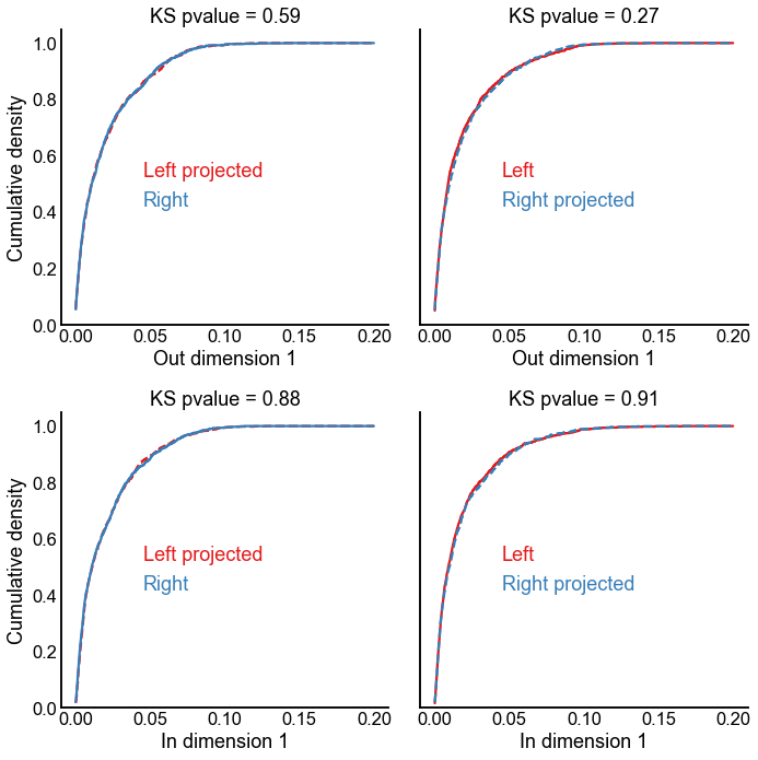
Run the projection experiment but without singular value scaling
fig, axs = plt.subplots(2, 2, figsize=(10, 10), sharey=True)
histplot_kws["bins"] = np.linspace(0, 0.2, 2000)
plot_dimension("Left", "out", axs[0, 0], unscale=True)
plot_dimension("Right", "out", axs[0, 1], unscale=True)
plot_dimension("Left", "in", axs[1, 0], unscale=True)
plot_dimension("Right", "in", axs[1, 1], unscale=True)
plt.tight_layout()
stashfig("projection-1d-comparison-unscaled")
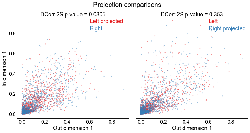
Test the 2-dimensional joint distributions
scatter_kws = dict(hue="hemisphere", palette=palette, s=10, linewidth=0, alpha=0.5)


def plot_paired_dimension(proj, ax, unscale=False):
    left_text = "Left"
    right_text = "Right"
    x_left = "out_1d"
    y_left = "in_1d"
    x_right = "out_1d"
    y_right = "in_1d"

    if proj == "Left":
        x_left += "_proj"
        y_left += "_proj"
        left_text += " projected"
    else:
        x_right += "_proj"
        y_right += "_proj"
        right_text += " projected"

    if unscale:
        x_left += "_unscale"
        x_right += "_unscale"
        y_left += "_unscale"
        y_right += "_unscale"

    left_df = embedding_1d_df[embedding_1d_df["hemisphere"] == "Left"]
    right_df = embedding_1d_df[embedding_1d_df["hemisphere"] == "Right"]

    sns.scatterplot(data=left_df, x=x_left, y=y_left, ax=ax, **scatter_kws)
    sns.scatterplot(data=right_df, x=x_right, y=y_right, ax=ax, **scatter_kws)
    ax.get_legend().remove()
    xlim = ax.get_xlim()
    ylim = ax.get_ylim()
    maxlim = max(xlim[1], ylim[1])
    minlim = min(xlim[0], ylim[0])
    xlim = (minlim, maxlim)
    ylim = (minlim, maxlim)
    ax.set(xlabel="Out dimension 1", ylabel="In dimension 1", ylim=ylim, xlim=xlim)
    ax.text(0.65, 0.95, left_text, color=palette["Left"], transform=ax.transAxes)
    ax.text(0.65, 0.88, right_text, color=palette["Right"], transform=ax.transAxes)

    left_data = left_df[[x_left, y_left]].values
    right_data = right_df[[x_right, y_right]].values
    test_results = run_test(left_data, right_data)
    pvalue = test_results["pvalue"]
    ax.set_title(f"DCorr 2S p-value = {pvalue:.3g}")


fig, axs = plt.subplots(1, 2, figsize=(12, 6), sharex=True, sharey=True)
plot_paired_dimension("Left", axs[0], unscale=False)
plot_paired_dimension("Right", axs[1], unscale=False)
plt.tight_layout()
fig.suptitle("Projection comparisons", y=1.03)
stashfig("projection-2d-comparison")
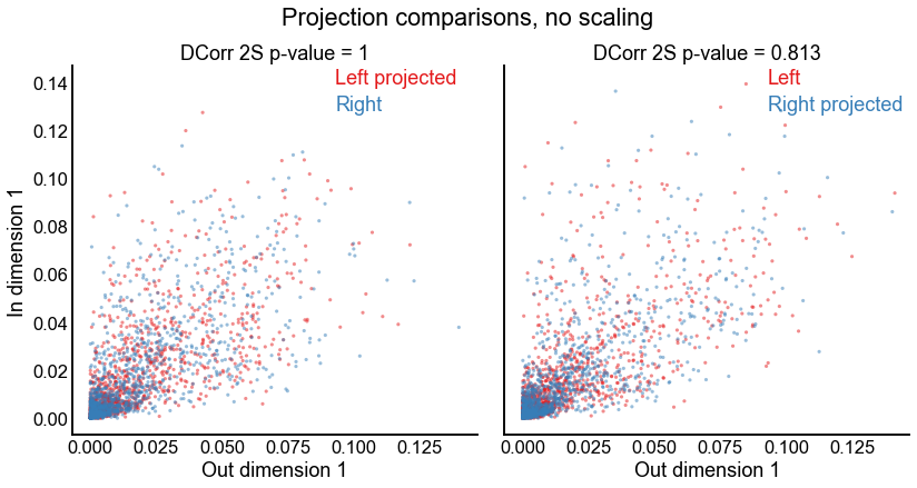
Test the 2-dimensional joints but without singular value scaling
fig, axs = plt.subplots(1, 2, figsize=(12, 6), sharex=True, sharey=True)
plot_paired_dimension("Left", axs[0], unscale=True)
plot_paired_dimension("Right", axs[1], unscale=True)
plt.tight_layout()
fig.suptitle("Projection comparisons, no scaling", y=1.03)
stashfig("projection-2d-comparison-unscaled")
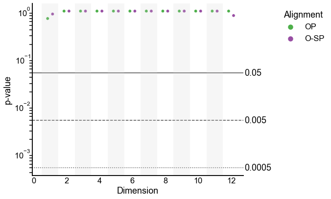
A “corrected” version of this test
We saw above that the alignment makes a huge difference in the outcome of the test. One possible way to fix this is to use a higher embedding dimension where the alignment is good, and then perform our test for varying numbers of kept dimensions (just like we did above where we aligned in \(d=8\) and tested the first \(d=1\) dimensions).
In this case, I use \(d=12\) as the alignment dimension, and test for \(d=1\), \(d=2\) etc. Note that testing at \(d=2\) means testing on the first 2 dimensions, not the second dimension alone.
align_n_components = (
    12  # this is one of the dimensions where we failed to reject before
)
op_left_out_latent, sp_left_out_latent = run_alignments(
    left_out_latent[:, :align_n_components], right_out_latent[:, :align_n_components]
)
op_left_in_latent, sp_left_in_latent = run_alignments(
    left_in_latent[:, :align_n_components], right_in_latent[:, :align_n_components]
)
rows = []
for n_components in np.arange(1, align_n_components + 1):
    left_out = op_left_out_latent.copy()[:, :n_components]
    left_in = op_left_in_latent.copy()[:, :n_components]
    right_out = right_out_latent[:, :align_n_components].copy()[:, :n_components]
    right_in = right_in_latent[:, :align_n_components].copy()[:, :n_components]

    left_composite_latent = np.concatenate((left_out, left_in), axis=1)
    right_composite_latent = np.concatenate((right_out, right_in), axis=1)

    run_test(
        left_composite_latent,
        right_composite_latent,
        rows,
        info={"alignment": "OP", "n_components": n_components},
    )

    left_out = sp_left_out_latent.copy()[:, :n_components]
    left_in = sp_left_in_latent.copy()[:, :n_components]
    left_composite_latent = np.concatenate((left_out, left_in), axis=1)

    run_test(
        left_composite_latent,
        right_composite_latent,
        rows,
        info={"alignment": "O-SP", "n_components": n_components},
    )

corrected_results = pd.DataFrame(rows)
Plot the results of the corrected version which starts from a good alignment
Here I plot the results only for orthogonal Procrustes. The behavior of the p-values is much closer to what we would have expected.
plot_pvalues(corrected_results)
End
elapsed = time.time() - t0
delta = datetime.timedelta(seconds=elapsed)
print("----")
print(f"Script took {delta}")
print(f"Completed at {datetime.datetime.now()}")
print("----")
----
Script took 0:14:32.475558
Completed at 2021-03-15 11:13:34.544446
----