Multiple Network Models
Contents
4.7. Multiple Network Models#
Up to this point, you have studied network models which are useful for a single network. What do you do if you have multiple networks?
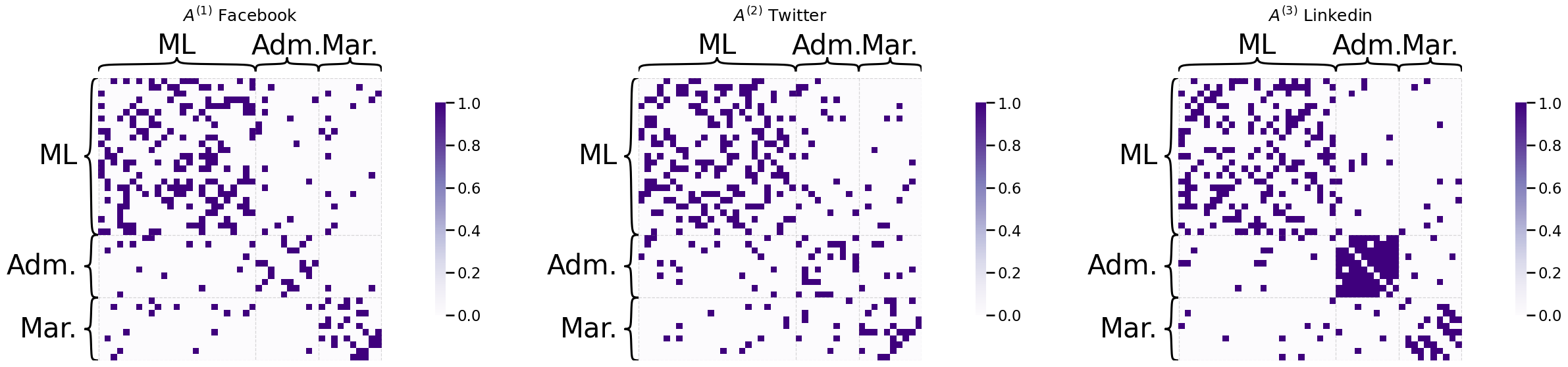
Let’s imagine that you have a company with \(45\) total employees. \(10\) of these employees are company administrative executives, \(25\) of these employees are network machine learning experts, and \(10\) of these employees are marketing experts. You study the social media habits of your employees on Facebook, Twitter, and Linkedin. For a given social networking site, an edge is said to exist between a pair of employees if they are connected on the social media site (by being friends, following one another, or being connected, respectively). As it turns out, individuals tend to most closely associate with the colleagues whom they work most closely: you might expect some sort of community structure to your network, wherein network machine learning experts are more connected with network machine learning experts, marketing experts are more connected with marketing experts, so on and so forth. What you will see below is that all of the networks appear to have the same community organization, though on Linkedin, you see that the administrative executives tend to be a little more connected. This is reflected in the fact that there are more connections between Adm. members on Linkedin:
from graphbook_code import heatmap
from graspologic.simulations import sbm
import numpy as np
import matplotlib.pyplot as plt

K = 3

B1 = np.zeros((K,K))

B1[0,0] = 0.3
B1[0,1] = .05
B1[1,0] = .05
B1[0,2] = .05
B1[2,0] = .05
B1[1,1] = 0.3
B1[1,2] = .05
B1[2,1] = .05
B1[2,2] = 0.3

B2 = B1

B3 = np.copy(B1)
B3[1,1] = 0.9

ns = [25, 10, 10]
A1 = sbm(n=ns, p=B1, directed=False, loops=False)
ys = ["ML" for i in range(0, ns[0])] + ["Adm." for i in range(ns[0],ns[0] + ns[1])] + ["Mar." for i in range(ns[0] + ns[1],ns[0] + ns[1] + ns[2])]

A2 = sbm(n=ns, p=B2, directed=False, loops=False)

A3 = sbm(n=ns, p=B3, directed=False, loops=False)

fig, axs = plt.subplots(1,3, figsize=(30, 6))

heatmap(A1, ax=axs[0], title="$A^{(1)}$ Facebook", color="sequential", xticklabels=False, yticklabels=False, inner_hier_labels=ys);

heatmap(A2, ax=axs[1], title="$A^{(2)}$ Twitter", color="sequential", xticklabels=False, yticklabels=False, inner_hier_labels=ys);

heatmap(A3, ax=axs[2], title="$A^{(3)}$ Linkedin", color="sequential", xticklabels=False, yticklabels=False, inner_hier_labels=ys);
Remember that a random network has an adjacency matrix denoted by a boldfaced uppercase \(\mathbf A\), and has network samples \(A\) (which you just call “networks”). When you have multiple networks, you will need to be able to index them individually. For this reason, in this section, you will use the convention that a random network’s adjacency matrix is denoted by a boldfaced uppercase \(\mathbf A^{(m)}\), where \(m\) tells you which network in your collection you are talking about. The capital letter \(M\) defines the total number of random networks in your collection. In your social network example, since you have connection networks for \(3\) sites, \(N\) is \(3\). When you use the letter \(m\) itself, you will typically be referring to an arbitrary random network among the collection of random networks, where \(m\) is between \(1\) and \(N\). When you have \(M\) total networks, you will write down the entire collection of random networks using the notation \(\left\{\mathbf A^{(1)}, ..., \mathbf A^{(M)}\right\}\). With what you already know, for a random network \(\mathbf A^{(m)}\), you would be able to use a single nework model to describe \(\mathbf A^{(m)}\). This means, for instance, if you thought that each social network could be represented by a different RDPG, that you would have a different latent position matrix \(X^{(m)}\) to define each of the \(30\) networks. In symbols, you would write that each \(\mathbf A^{(m)}\) is an RDPG random nework with latent position matrix \(X^{(m)}\). What is the problem with this description?
What this description lacks is that the three networks share a lot of common information. You might expect that, on some level, the latent position matrices should also show some sort of common structure. However, since you used a unique latent position matrix \(X^{(m)}\) for each random network \(\mathbf A^{(m)}\), you have inherently stated that you think that the networks have completely distinct latent position matrices. If you were to perform a task downstream, such as whether you could identify which employees are in which community, you would have to analyze each latent position matrix individually, and you would not be able to learn a latent position matrix with shared structure across the three networks. Before you jump into multiple network models, let’s provide some context as to how you will build these up.
In the below descriptions, you will tend to build off the Random Dot Product Graph (RDPG), and closely related variations of it. Why? Well, as it turns out, the RDPG is extremely flexible, in that you can represent both ER and SBMs as RDPGs, too. You’ll remember from The IER network unifies independent-edge random networks, as it is the most general independent-edge random network model. What this means is that all models discussed so far, and many not discussed but found in the appendix, can be conceptualized as special cases of the IER network. Stated in other words, a probability matrix is the fundamental unit necessary to describe an independent-edge random network model. For the models covered so far, all GRDPGs are IER networks (by taking P to be XY^\top), all RDPGs are GRDPGs (by taking the right latent positions Y to be equal to the left latent positions X), all SBMs are RDPGs, and all ERs are SBMs, whereas the converses in general are not true. that the ER network was a special case of the SBM and SBMs were special cases of RDPG networks, so the RDPG can describe any network which is an RDPG, an SBM, or an ER random network. This means that building off the RDPG gives you multiple random network models that will be inherently flexible. Further, as you will see in the later section on Learning Network Representations, the RDPG is extremely well-suited for the situation in which you want to analyze SBMs, but do not know which communities the nodes are in ahead of time. This situation is extremely common across numerous disciplines of network machine learning, such as social networking, neuroscience, and many other fields.
So, how can you model your collection of random networks with shared structure?
4.7.1. Joint Random Dot Product Graphs (JRDPG) Model#
In our example on social networks, notice that the Facebook and Twitter connections do not look too qualitatively different. It looks like they have relatively similar connectivity patterns between the different employee working groups, and you might even think that the underlying random network that governs these two social networks are identical. In statisical science, when we have a collection of \(M\) random networks that have the same underlying random process, we describe this with the term homogeneity. Let’s put what this means into context using your coin flip example. If a pair of coins are homogeneous, this means that the probability that they land on heads is identical. Likewise, this intuition extends directly to random networks.
A homogeneous collection of independent-edge random networks \(\left\{\mathbf A^{(1)}, ..., \mathbf A^{(M)}\right\}\) is one in which all of the \(M\) random networks have the same probability matrix, and consequently have the same distribution (statistically, the term is identically distributed). Remember that the probability matrix \(P^{(m)}\) is the matrix whose entries \(p^{(m)}_{ij}\) indicate the probability that an edge exists between nodes \(i\) and \(j\). This is because the probability matrix is the fundamental unit which can be used to describe independent-edge random networks, as we learned in Inhomogeneous Erdos Renyi (IER) Random Network Model. On the other hand, a heterogeneous collection of random networks is a collection of networks \(\left\{\mathbf A^{(1)}, ..., \mathbf A^{(M)}\right\}\) is one in which the probability matrices are not the same for all of the \(M\) networks, and hence, they are not identically distributed.
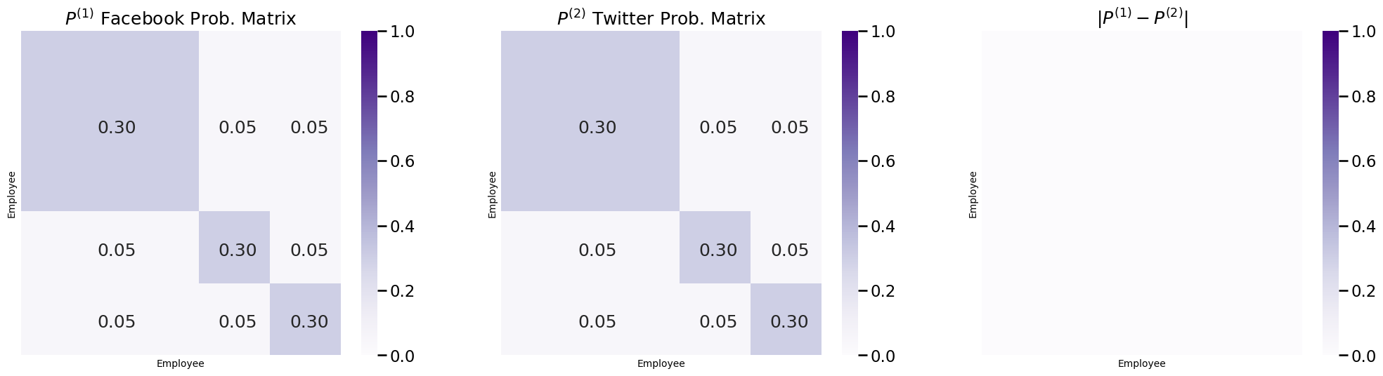
The probability matrices \(P^{(1)}\) and \(P^{(2)}\) for the random networks \(\mathbf A^{(1)}\) and \(\mathbf A^{(2)}\) for Facebook and Twitter from the example we introduced above are shown in the following figure. You can also show the difference between the two probability matrices, to make really clear that they are the same:
import seaborn as sns
from graphbook_code import cmaps
import pandas as pd

def p_from_block(B, ns):
    P = np.zeros((np.sum(ns), np.sum(ns)))
    ns_cumsum = np.append(0, np.cumsum(ns))
    for k, n1 in enumerate(ns_cumsum[0:(len(ns_cumsum)-1)]):
        for l, n2 in enumerate(ns_cumsum[k:(len(ns_cumsum)-1)]):
            P[ns_cumsum[k]:ns_cumsum[k+1], ns_cumsum[l+k]:ns_cumsum[l+k+1]] = B[k,l+k]
            P[ns_cumsum[l+k]:ns_cumsum[l+k+1],ns_cumsum[k]:ns_cumsum[k+1]] = B[l+k,k]
    return P

P1 = p_from_block(B1, ns)
U1, S1, V1 = np.linalg.svd(P1)
X1 = U1[:,0:3] @ np.sqrt(np.diag(S1[0:3]))

P2 = p_from_block(B2, ns)
U2, S2, V2 = np.linalg.svd(P2)
X2 = U2[:,0:3] @ np.sqrt(np.diag(S2[0:3]))

P3 = p_from_block(B3, ns)
U3, S3, V3 = np.linalg.svd(P3)
X3 = U3[:,0:3] @ np.sqrt(np.diag(S3[0:3]))

def plot_prob_block_annot(X, title="", nodename="Employee", nodetix=None,
             nodelabs=None, ax=None, annot=True):
    if (ax is None):
        fig, ax = plt.subplots(figsize=(8, 6))

    with sns.plotting_context("talk", font_scale=1):
        if annot:
            X_annot = np.empty(X.shape, dtype='U4')
            X_annot[13, 13] = str("{:.3f}".format(X[13,13]))
            X_annot[30, 30] = str("{:.3f}".format(X[30,30]))
            X_annot[40,40] = str("{:.3f}".format(X[40,40]))
            X_annot[13, 30] = str("{:.3f}".format(X[13,30]))
            X_annot[30,13] = str("{:.3f}".format(X[30,13]))
            X_annot[13,40] = str("{:.3f}".format(X[23,40]))
            X_annot[40,13] = str("{:.3f}".format(X[40,13]))
            X_annot[30,40] = str("{:.3f}".format(X[30,40]))
            X_annot[40,30] = str("{:.3f}".format(X[40,30]))
            ax = sns.heatmap(X, cmap="Purples",
                            ax=ax, cbar_kws=dict(shrink=1), yticklabels=False,
                            xticklabels=False, vmin=0, vmax=1, annot=pd.DataFrame(X_annot),
                            fmt='')
        else:
            ax = sns.heatmap(X, cmap="Purples",
                            ax=ax, cbar_kws=dict(shrink=1), yticklabels=False,
                            xticklabels=False, vmin=0, vmax=1)
        ax.set_title(title)
        cbar = ax.collections[0].colorbar
        ax.set(ylabel=nodename, xlabel=nodename)
        if (nodetix is not None) and (nodelabs is not None):
            ax.set_yticks(nodetix)
            ax.set_yticklabels(nodelabs)
            ax.set_xticks(nodetix)
            ax.set_xticklabels(nodelabs)
        cbar.ax.set_frame_on(True)
    return

fig, axs = plt.subplots(1,3, figsize=(25, 6))
plot_prob_block_annot(P1, ax=axs[0], title="$P^{(1)}$ Facebook Prob. Matrix")
plot_prob_block_annot(P2, ax=axs[1], title="$P^{(2)}$ Twitter Prob. Matrix")
plot_prob_block_annot(np.abs(P1 - P2), ax=axs[2], annot=False, title="$|P^{(1)} - P^{(2)}|$")
The Joint Random Dot Product Graphs (JRDPG) is the simplest way you can extend the RDPG random network model to multiple random networks. The way you can think of the JRDPG model is that for each of your \(M\) total random neworks, the edges depend on a latent position matrix \(X\). You say that a collection of random networks \(\left\{\mathbf A^{(1)}, ..., \mathbf A^{(N)}\right\}\) with \(n\) nodes is \(JRDPG_{n,M}(X)\) if each random network \(\mathbf A^{(m)}\) is \(RDPG_n(X)\) and if the \(N\) networks are independent. The joint random dot product graph model is formally described by [3], and has many connections with the omnibus embedding [2], which you will learn about in Section 5.4.
4.7.1.1. The JRDPG model does not allow you to convey unique aspects about the networks#
Under the JRDPG model, each of the \(M\) random networks share the same latent position matrix. Remember that for an RDPG, the probability matrix \(P = XX^\top\). This means that for all of the \(M\) networks, \(P^{(m)} = XX^\top\) under the JRDPG model. hence, \(P^{(1)} = P^{(2)} = ... = P^{(M)}\), and all of the probability matrices are identical! This means that the \(M\) random networks are homogeneous. Consequently, the JRDPG can be literally thought of as \(M\) independent RDPGs.
For an RDPG, since \(P = XX^\top\), the probability matrix depends only on the latent positions \(X\). This means that you can tell whether a collection of networks are homogeneous just by looking at the latent position matrices! It turns out that the random networks underlying the samples for the social networks in your given example were just SBMs. From the section on Random Dot Product Graphs (RDPG), you learned that SBMs are just RDPGs with a special latent position matrix. Let’s try this first by looking at latent position matrices for \(\mathbf A^{(1)}\) and \(\mathbf A^{(2)}\) from the random networks for Facebook and Twitter first which were used to generate our network samples:
from numpy.linalg import svd

def plot_latent(X, title="", nodename="Employee", ylabel="Latent Dimension",
                nodetix=None, vmin=None, vmax=None, nodelabs=None, ax=None, dimtix=None, dimlabs=None):
    if ax is None:
        fig, ax = plt.subplots(figsize=(6, 6))

    with sns.plotting_context("talk", font_scale=1):
        lim_max = np.max(np.abs(X))
        if vmin is None:
            vmin = -lim_max
        if vmax is None:
            vmax = lim_max
        X_annot = np.empty((45, 3), dtype='U6')
        X_annot[13,0] = str("{:.3f}".format(X[13,0]))
        X_annot[30,0] = str("{:.3f}".format(X[30,0]))
        X_annot[40,0] = str("{:.3f}".format(X[40,0]))
        X_annot[13,1] = str("{:.3f}".format(X[13,1]))
        X_annot[30,1] = str("{:.3f}".format(X[30,1]))
        X_annot[40,1] = str("{:.3f}".format(X[40,1]))
        X_annot[13,2] = str("{:.3f}".format(X[13,2]))
        X_annot[30,2] = str("{:.3f}".format(X[30,2]))
        X_annot[40,2] = str("{:.3f}".format(X[40,2]))
        ax = sns.heatmap(X, cmap=cmaps["divergent"],
                        ax=ax, cbar_kws=dict(shrink=1), yticklabels=False,
                        xticklabels=False, vmin=vmin, vmax=vmax,
                        annot=X_annot, fmt='')
        ax.set_title(title)
        cbar = ax.collections[0].colorbar
        ax.set(ylabel=nodename, xlabel=ylabel)
        if (nodetix is not None) and (nodelabs is not None):
            ax.set_yticks(nodetix)
            ax.set_yticklabels(nodelabs)
        if (dimtix is not None) and (dimlabs is not None):
            ax.set_xticks(dimtix)
            ax.set_xticklabels(dimlabs)
        cbar.ax.set_frame_on(True)
    return

fig, axs = plt.subplots(1,3, figsize=(20, 6))
vmin = np.min([X1,X2,X3]); vmax = np.max([X1, X2, X3])
plot_latent(X1, nodetix=[0,24,34,44], vmin=vmin, vmax=vmax, nodelabs=["1", "25", "35", "45"],
            dimtix=[0.5,1.5,2.5], ax=axs[0], dimlabs=["1", "2", "3"], title="$X^{(1)}$ Facebook LPM")
plot_latent(X2, nodetix=[0,24,34,44], nodelabs=["1", "25", "35", "45"],
            dimtix=[0.5,1.5,2.5], ax=axs[1], vmin=vmin, vmax=vmax, dimlabs=["1", "2", "3"], title="$X^{(2)}$ Twitter LPM")
plot_latent(np.abs(X1 - X2), nodetix=[0,24,34,44], vmin=vmin, vmax=vmax, nodelabs=["1", "25", "35", "45"],
            dimtix=[0.5,1.5,2.5], ax=axs[2], dimlabs=["1", "2", "3"], title="$|X^{(1)} - X^{(2)}|$")
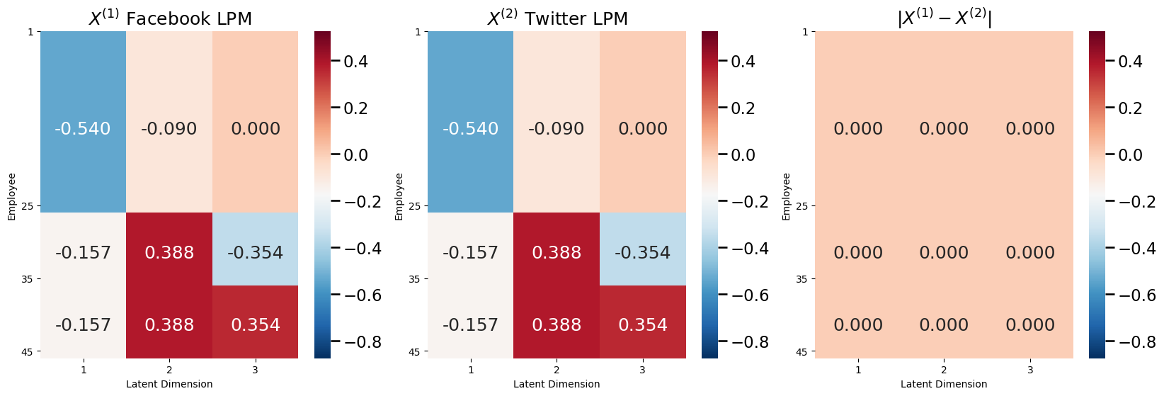
So the latent position matrices for Facebook and Twitter are exactly identical. Therefore, the collection of random networks \(\left\{\mathbf A^{(1)}, \mathbf A^{(2)}\right\}\) are homogeneous, and you could model this pair of networks using the JRDPG.
What about Linkedin? Well, as it turns out, Linkedin had a different latent position matrix from both Facebook and Twitter:
fig, axs = plt.subplots(1,3, figsize=(20, 6))
vmin = np.min([X1,X2,X3]); vmax = np.max([X1, X2, X3])
plot_latent(X1, nodetix=[0,24,34,44], vmin=vmin, vmax=vmax, nodelabs=["1", "25", "35", "45"],
            dimtix=[0.5,1.5,2.5], ax=axs[0], dimlabs=["1", "2", "3"], title="$X^{(1)}$ Facebook LPM")
plot_latent(X3, nodetix=[0,24,34,44], nodelabs=["1", "25", "35", "45"],
            dimtix=[0.5,1.5,2.5], ax=axs[1], vmin=vmin, vmax=vmax, dimlabs=["1", "2", "3"], title="$X^{(3)}$ Linkedin LPM")
plot_latent(np.abs(X1 - X3), nodetix=[0,24,34,44], vmin=vmin, vmax=vmax, nodelabs=["1", "25", "35", "45"],
            dimtix=[0.5,1.5,2.5], ax=axs[2], dimlabs=["1", "2", "3"], title="$|X^{(1)} - X^{(3)}|$")
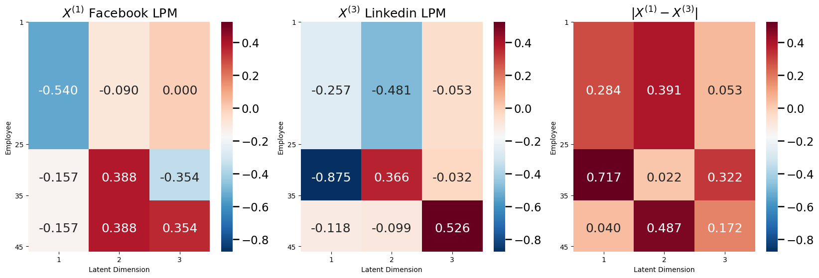
So, \(\mathbf A^{(1)}\) and \(\mathbf A^{(3)}\) do not have the same latent position matrices. This means that the collections of random networks \(\left\{\mathbf A^{(1)}, \mathbf A^{(3)}\right\}\), \(\left\{\mathbf A^{(2)}, \mathbf A^{(3)}\right\}\), and \(\left\{\mathbf A^{(1)}, \mathbf A^{(2)}, \mathbf A^{(3)}\right\}\) are heterogeneous, because their probability matrices will be different. So, unfortunately, the JRDPG cannot handle the hetereogeneity between the random networks of Facebook and Twitter with the random network for Linkedin. To remove this restrictive homogeneity property of the JRDPG, you can turn to the single network model you just learned about: the Independent Erdos Renyi (IER) random network. Next, you will see how the IER random network can be used in conjunction with the COSIE model to allow you to capture this heterogeneity.
4.7.2. Common Subspace Independent Edge (COSIE) Model#
In your example on social networks, notice that the Facebook and Linkedin connections looked relatively similar, but had an important difference: on Linkedin, there was an administrative meeting, and the employees on the administrative team exchanged far more connections than usual among one another. It turns out that, in fact, the random networks \(\mathbf A^{(1)}\) and \(\mathbf A^{(3)}\) which underly the social networks \(A^{(1)}\) and \(A^{(3)}\) were also different, because the probability matrices were different:
fig, axs = plt.subplots(1,3, figsize=(25, 6))
plot_prob_block_annot(P1, ax=axs[0], title="$P^{(1)}$ Facebook Prob. Matrix")
plot_prob_block_annot(P3, ax=axs[1], title="$P^{(3)}$ Linkedin Prob. Matrix")
plot_prob_block_annot(np.abs(P1 - P3), ax=axs[2], annot=True, title="$|P^{(1)} - P^{(3)}|$")
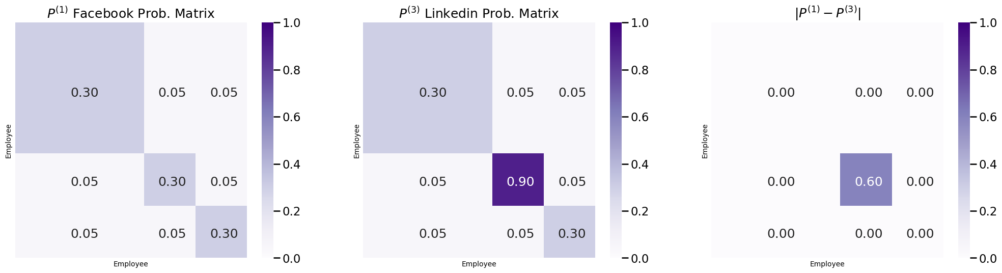
Notice that the difference in the probability of a connection being shared between the members of the administrative team is \(0.6\) higher in the probability matrix for Linkedin than for Facebook. This is because the random networks \(\mathbf A^{(1)}\) and \(\mathbf A^{(3)}\) are heterogeneous. To reflect this heterogeneity, we turn to the COmmon Subspace Independent Edge (COSIE) model.
4.7.2.1. The COSIE Model is defined by a collection of score matrices and a shared low-rank subspace#
Even though \(P^{(1)}\) and \(P^{(3)}\) are not identical, you can see they still share some structure: the employee teams are the same between the two social networks, and much of the probability matrix is unchanged. For this reason, it will be useful for you to have a network model which allows you to convey some shared structure, but still lets you convey aspects of the different networks which are unique. Ultimately, our goal with network modelling is to make sense of the networks we observe downstream, which is difficult to do when there are too many things you need to estimate or think about simultaneously. This shared structure will allow you to borrow strength when you estimate, which will allow you to feasibly estimate all of the ingredients you will need to describe COSIE networks. The COSIE model will accomplish this using a shared latent position matrix to describe the similarities, and unique score matrices to describe the differences, for each of the random networks. Let’s learn about what these are.
4.7.2.1.1. The Shared Latent Position Matrix Describes Similarities#
The shared latent position matrix for the COSIE model is quite similar to the latent position matrix for an RDPG. Like the latent position matrix, the shared latent position matrix \(V\) is a matrix with \(n\) rows (one for each node) and \(d\) columns. The \(d\) columns behave very similarly to the \(d\) columns for the latent position matrix of an RDPG, and \(d\) is referred to as the latent dimensionality of the COSIE random networks. Like before, each row of the shared latent position matrix \(\vec v_i\) will denote the shared latent position vector for node \(i\).
We will also add an additional restriction to \(V\): it will be a matrix with orthonormal columns. What this means is that for each column of \(V\), the dot product of the column with itself is \(1\), and the dot product of the column with any other column is \(0\). This has the implication that \(V^\top V = I\), the identity matrix. All this has the effect of doing is it gives you a sense of uniform scale for all of the columns (scale \(1\)) of the latent position matrix. This has the effect of allowing the other component, the score matrix, to be interpretable, which you will learn more about in the next subsection.
The shared latent position matrix conveys the common structure between the COSIE random networks, and will be a parameter for each of the neworks. Remember that with the \(JRDPG_n(X)\) model, you were able to express the homogeneity of the social networks on Facebook and Twitter, but you could not capture the heterogeneity of the social nework on Linkedin. However, you want the shared latent position matrix \(V\) to convey the commonality among the three social networks; that is, that the employees are always working on the same employee teams. Let’s take a look at the shared latent position matrix \(V\) for the social network example:
from graspologic.embed import MultipleASE as MASE

embedder = MASE(n_components=3)
V = embedder.fit_transform([P1, P2, P3])

plot_latent(V, nodetix=[0,24,34,44], nodelabs=["1", "25", "35", "45"],
            dimtix=[0.5,1.5,2.5], dimlabs=["1", "2", "3"], title="$V$, Shared Latent Positions")
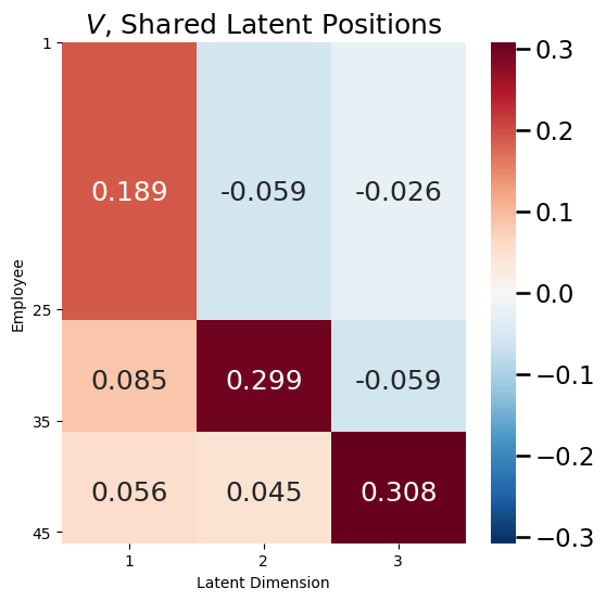
\(V\) reflects the fact that the first \(25\) employees are the ML experts, and all \(25\) have the same latent position vector. The next \(10\) employees are the administrative members, and share a different latent position vector from the ML experts. Finally, the last \(10\) employees are the marketing members, share a different latent position vector from the ML experts and the administrative team. In this way, the orthonormal matrix \(V\) has conveyed the community structure (the employee roles and who they tend to connect among) that is shared across all three days.
4.7.2.1.2. Score Matrices Describe Differences#
The score matrices for the COSIE random networks essentially tell you how to assemble the shared latent position matrix to obtain the unique probability matrix for each network. The score matrix \(R^{(m)}\) for a random network \(m\) is a matrix with \(d\) columns and \(d\) rows. Therefore, it is a square matrix whose number of dimensions is equal to the latent dimensionality of the COSIE random networks.
The probability matrix for each network under the COSIE model is the matrix:
When you look at this expression, you can understand it a little bit better by focusing on the first multiplication, the term \(VR^{(m)}\). You are basically taking the shared latent position matrix, and using the scores to express which latent position vectors are more, or less, important in the probability matrix \(P^{(m)}\). In this sense, the score matrix tells you which combinations of latent positions determine the unique features of heterogeneous probability matrices.
In the social network example, you want the score matrices to indicate that Facebook and Twitter share a probability matrix, but Facebook and Linkedin do not. Consequently, you would expect that the score matrices from Facebook and Twitter should be the same, but the score matrix for Linkedin will be different:
def plot_score(X, title="", blockname="Employee Group", blocktix=[0.5, 1.5, 2.5],
               blocklabs=["ML", "Adm.", "Mark."], ax=None, vmin=0, vmax=1):
    if ax is None:
        fig, ax = plt.subplots(figsize=(8, 6))

    with sns.plotting_context("talk", font_scale=1):
        ax = sns.heatmap(X, cmap="Purples",
                        ax=ax, cbar_kws=dict(shrink=1), yticklabels=False,
                        xticklabels=False, vmin=vmin, vmax=vmax, annot=True)
        ax.set_title(title)
        cbar = ax.collections[0].colorbar
        ax.set(ylabel=blockname, xlabel=blockname)
        ax.set_yticks(blocktix)
        ax.set_yticklabels(blocklabs)
        ax.set_xticks(blocktix)
        ax.set_xticklabels(blocklabs)
        cbar.ax.set_frame_on(True)
    return

vmin=np.min(embedder.scores_); vmax = np.max(embedder.scores_)

fig, axs = plt.subplots(1,3, figsize=(25, 6))
R1 = embedder.scores_[0,:,:]
R2 = embedder.scores_[1,:,:]
R3 = embedder.scores_[2,:,:]

plot_score(R1, ax=axs[0], vmin=vmin, vmax=vmax, title="$R^{(1)}$ Facebook Scores")
plot_score(R2, ax=axs[1], vmin=vmin, vmax=vmax, title="$R^{(2)}$ Twitter Scores")
plot_score(R3, ax=axs[2], vmin=vmin, vmax=vmax, title="$R^{(3)}$ Linkedin Scores")
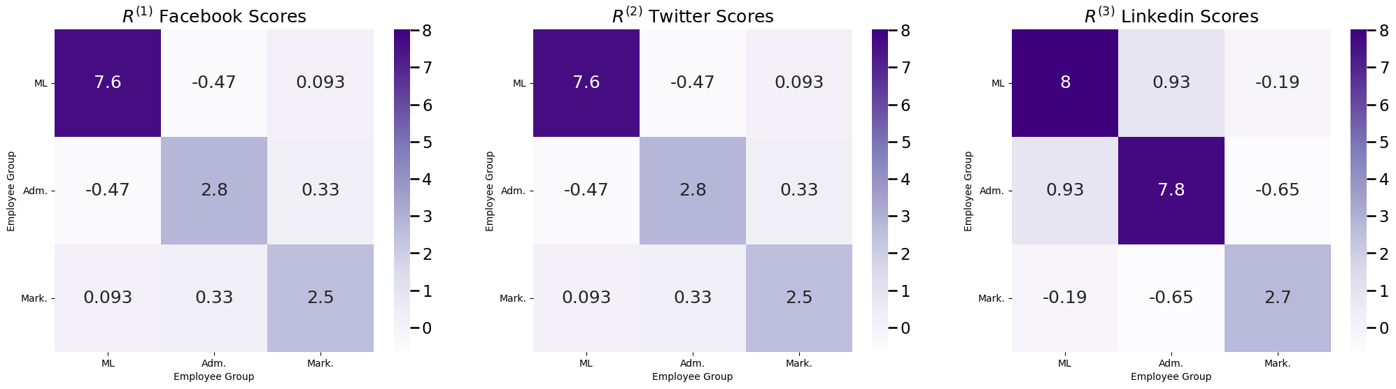
As you can see, the scores \(R^{(1)}\) and \(R^{(2)}\) are the same for Facebook and Twitter, but different for \(R^{(3)}\) Linkedin.
Finally, let’s relate all of this back to the COSIE model. The way you can think about the COSIE model is that for each random network that you have, the probability matrix \(P^{((m)}\) depends on the shared latent position matrix \(V\) and the score matrix \(R^{(m)}\). The probability matrix \(P^{(m)}\) for the \(m^{th}\) random network is defined so that \(P^{(m)} = VR^{(m)}V^\top\). This means that each entry \(p_{ij}^{(m)} = \vec v_i^\top R^{(m)} \vec v_j\). We say that a collection of random networks \(\left\{\mathbf A^{(1)}, ..., \mathbf A^{(M)}\right\}\) with \(n\) nodes is \(COSIE_{n,M}\left(V, \left\{R^{(1)},...,R^{(M)}\right\}\right)\) if each random network \(\mathbf A^{(m)}\) is \(IER(P^{(m)})\). Stated another way, each of the \(M\) random networks share the same orthonormal matrix \(V\), but a unique score matrix \(R^{(m)}\). This allows the random networks to share some underlying structure (which is conveyed by \(V\)) but each random network still has a combination of this shared structure (conveyed by \(R^{(m)}\)).
Since the probability matrix \(P^{(m)} = VR^{(m)}V^\top\), you can see that two random networks with the same score matrix will be homogeneous (identically distributed), and two random networks with different score matrices will be heterogeneous (not identically distributed). In this way, you are able to capture the homogeneity between the random networks for Facebook and Twitter connections, while also capturing the heterogeneity between the random networks for Facebook and Linkedin connections. The COSIE model is described by [3], and has direct connections with the multiple adjacency spectral embedding, which you will learn about in Section 5.4.
4.7.3. Correlated Network Models#
Finally, we get to a special case of network models, known as correlated network models. Let’s say that you have a group of people in a city, and you know that each person in your group have both a Facebook and a Twitter account. The nodes in your network are the people who possess accounts. The first network consists of Facebook connections among the people, where an edge exists between two people if they are friends on Facebook. The second network consists of Twitter connections among the people, where an edge exists between two people if they follow one another on Twitter. You think that if two people are friends on Facebook, there is a good chance that they follow one another on Twitter, and vice versa. How do you reflect this similarity through a multiple network model?
At a high level, network correlation between a pair of networks describes the property that the existence of edges in one network provides you with some level of information about edges in the other network, much like the Facebook/Twitter example that you just saw. In this book, we will focus on the \(\rho\)-correlated network models. What the \(\rho\)-correlated network models focus on is that given two random networks with the same number of nodes, each edge has a correlation of \(\rho\) between the two networks. To define this a little more rigorously, a pair of random networks \(\mathbf A^{(1)}\) and \(\mathbf A^{(2)}\) are called \(\rho\)-correlated if all of the edges across both networks are mutually independent, except that for all pairs of indices \(i\) and \(j\), \(corr(\mathbf a_{ij}^{(1)}, \mathbf a_{ij}^{(2)}) = \rho\), where \(corr(\mathbf x, \mathbf y)\) is the Pearson correlation between two random variables \(\mathbf x\) and \(\mathbf y\). In our example, this means that whether two people are friends on Facebook is correlated with whether they are following one another on Twitter.
At a high level, the Pearson correlation describes whether one variable being large/small gives information that the other variable is large/small (positive correlation, between \(0\) and \(1\)) or whether one variable being large/small gives information that the other variable will be small/large (negative correlation, between \(-1\) and \(0\)). If the two networks are positively correlated and you know that one of the edges \(\mathbf a_{ij}^{(1)}\) has a value of one, then you have information that \(\mathbf a_{ij}^{(2)}\) might also be one, and vice-versa for taking values of zero. If the two networks are negatively correlated and you know that one of the edges \(\mathbf a_{ij}^{(1)}\) has a value of one, then you have information that \(\mathbf a_{ij}^{(2)}\) might be zero, and vice-versa. If the two networks are not correlated (\(\rho = 0\)) you do not learn anything about edges of network two by looking at edges from network one.
4.7.3.1. \(\rho\)-Correlated RDPG#
The \(\rho\)-correlated RDPG is the most general correlated network model you will need for the purposes of this book, and is described by [4] and [5]. Remembering that both ER and SBM random networks are special cases of the RDPG (for a given choice of the latent position matrix), the \(\rho\)-correlated RDPG can therefore be used to construct \(\rho\)-correlated ER and \(\rho\)-correlated SBMs, too. The way you can think about the \(\rho\)-correlated RDPG is that like for the normal RDPG, a latent position matrix \(X\) with \(n\) rows and a latent dimensionality of \(d\) is used to define the edge-existence probabilities for the networks \(\mathbf A^{(1)}\) and \(\mathbf A^{(2)}\). We begin by defining that \(\mathbf A^{(1)}\) is \(RDPG_n(X)\). Next, we define the second network as follows. We use a coin for each edge \((i, j)\), which has a probability that depends on the values that the first network takes. If the edge \(\mathbf a_{ij}^{(1)}\) takes the value of one, then we use a coin which has a probability of landing on heads of \(\vec x_i^\top \vec x_j + \rho(1 - \vec x_i^\top \vec x_j)\). If the edge \(\mathbf a_{ij}^{(1)}\) takes the value of zero, then we use a coin which has a probability of landing on heads of \((1 - \rho)\vec x_i^\top \vec x_j\). We flip this coin, and if it lands on heads, then the edge \(\mathbf a_{ij}^{(2)}\) takes the value of one. If it lands on tails, then the edge \(\mathbf a_{ij}^{(2)}\) takes the value of zero. If \(\mathbf A^{(1)}\) and \(A^{(2)}\) are random networks which are \(\rho\)-correlated RDPGs with latent position matrix \(X\), we say that the pair \(\left\{\mathbf A^{(1)}, A^{(2)}\right\}\) are \(\rho-RDPG_n(X)\).
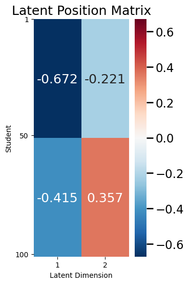
Fortunately, graspologic makes sampling \(\rho\)-correlated RDPGs relatively simple. Let’s say that in your Facebook/Twitter example, you have \(100\) people across two schools, like your standard example from the SBM section. The first \(50\) students attend school one, and the second \(50\) students attend school two. To recap, the latent position matrix looks like this:
import numpy as np
from numpy.linalg import svd

n = 100

# deine a probability matrix for a stochastic block model with two communities
# where the first 50 students are from community one and the second 50 students are
# from community two
P = np.zeros((n,n))
P[0:50,0:50] = .5
P[50:100, 50:100] = .3
P[0:50,50:100] = .2
P[50:100,0:50] = .2

# use the singular value decomposition to obtain the corresponding latent
# position matrix
U, S, V = svd(P)
X = U[:,0:2] @ np.sqrt(np.diag(S[0:2]))
from graphbook_code import cmaps
import matplotlib.pyplot as plt
import seaborn as sns

def plot_latent(X, title="", nodename="Student", ylabel="Latent Dimension",
                nodetix=None, nodelabs=None, dimtix=None, dimlabs=None):
    fig, ax = plt.subplots(figsize=(3, 6))

    with sns.plotting_context("talk", font_scale=1):
        lim_max = np.max(np.abs(X))
        vmin = -lim_max; vmax = lim_max
        X_annot = np.empty((100, 2), dtype='U6')
        X_annot[25,0] = str("{:.3f}".format(X[25,0]))
        X_annot[75,0] = str("{:.3f}".format(X[75,0]))
        X_annot[25,1] = str("{:.3f}".format(X[25,1]))
        X_annot[75,1] = str("{:.3f}".format(X[75,1]))
        ax = sns.heatmap(X, cmap=cmaps["divergent"],
                        ax=ax, cbar_kws=dict(shrink=1), yticklabels=False,
                        xticklabels=False, vmin=vmin, vmax=vmax,
                        annot=X_annot, fmt='')
        ax.set_title(title)
        cbar = ax.collections[0].colorbar
        ax.set(ylabel=nodename, xlabel=ylabel)
        if (nodetix is not None) and (nodelabs is not None):
            ax.set_yticks(nodetix)
            ax.set_yticklabels(nodelabs)
        if (dimtix is not None) and (dimlabs is not None):
            ax.set_xticks(dimtix)
            ax.set_xticklabels(dimlabs)
        cbar.ax.set_frame_on(True)
    return


ax = plot_latent(X, title="Latent Position Matrix", nodetix=[0, 49, 99],
              nodelabs=["1", "50", "100"], dimtix=[0.5,1.5], dimlabs=["1", "2"])
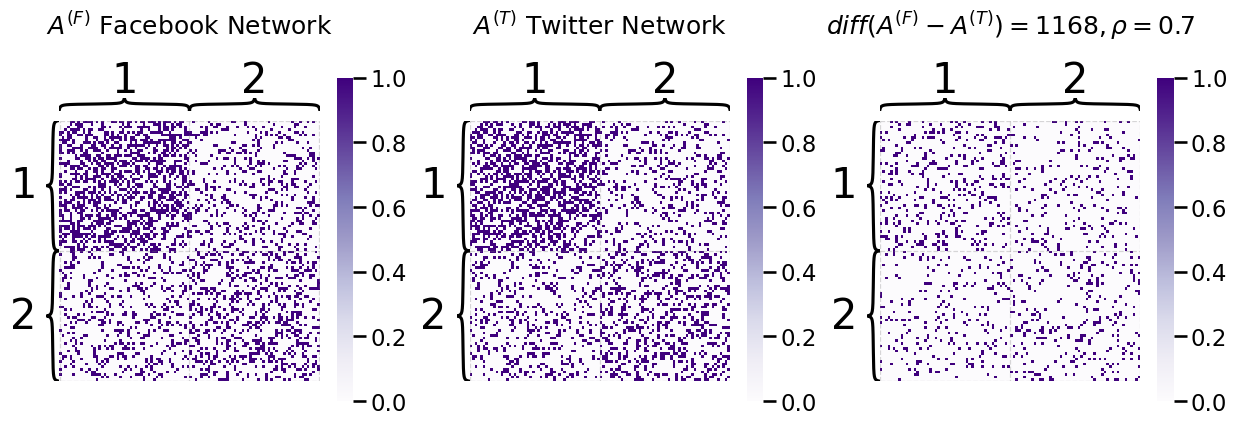
To sample two networks which are \(\rho\)-correlated SBMs, let’s assume that the correlation between the two networks is high, so you will let \(\rho = 0.7\). You use the graspologic function to obtain a sample for each network. You can look at a plot the two networks, as well as the edges which are different between the two networks. You can summarize this edge difference plot with \(diff(A^{(F)} - A^{(T)})\), which simply counts the number of edges which are different:
from graspologic.simulations import rdpg_corr

rho = 0.7
A_Facebook, A_Twitter = rdpg_corr(X, Y=None, r=rho, directed=False, loops=False)
fig, axs = plt.subplots(1,3, figsize=(15, 6))

ys = ["1" for i in range(0, 50)] + ["2" for i in range(0, 50)]

heatmap(A_Facebook, ax=axs[0], title="$A^{(F)}$ Facebook Network", color="sequential", xticklabels=False, yticklabels=False, inner_hier_labels=ys);

heatmap(A_Twitter, ax=axs[1], title="$A^{(T)}$ Twitter Network", color="sequential", xticklabels=False, yticklabels=False, inner_hier_labels=ys);

heatmap(np.abs(A_Facebook - A_Twitter), ax=axs[2], title="$diff(A^{(F)} - A^{(T)}) = %d, \\rho = 0.7$" % np.abs(A_Facebook - A_Twitter).sum(),
        color="sequential", xticklabels=False, yticklabels=False, inner_hier_labels=ys);
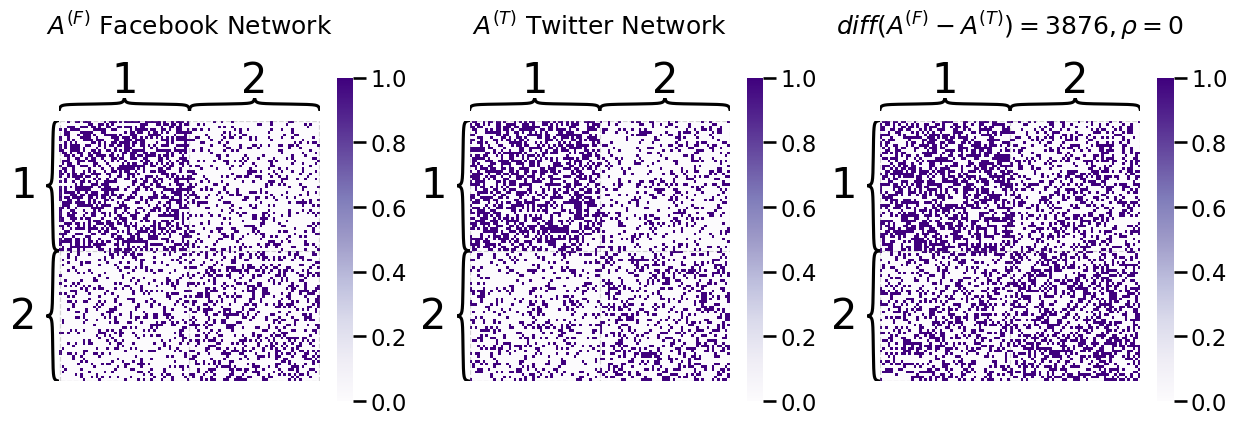
On the other hand, if the correlation were \(\rho = 0\) (the two networks are uncorrelated), you can see that the number of edges which are different is much higher:
rho = 0.0
A_Facebook, A_Twitter = rdpg_corr(X, Y=None, r=rho, directed=False, loops=False)
fig, axs = plt.subplots(1,3, figsize=(15, 6))

ys = ["1" for i in range(0, 50)] + ["2" for i in range(0, 50)]

heatmap(A_Facebook, ax=axs[0], title="$A^{(F)}$ Facebook Network", color="sequential", xticklabels=False, yticklabels=False, inner_hier_labels=ys);

heatmap(A_Twitter, ax=axs[1], title="$A^{(T)}$ Twitter Network", color="sequential", xticklabels=False, yticklabels=False, inner_hier_labels=ys);

heatmap(np.abs(A_Facebook - A_Twitter), ax=axs[2], title="$diff(A^{(F)} - A^{(T)}) = %d, \\rho = 0$" % np.abs(A_Facebook - A_Twitter).sum(),
        color="sequential", xticklabels=False, yticklabels=False, inner_hier_labels=ys);
4.7.4. References#
- 1
Avanti Athreya, Donniell E. Fishkind, Minh Tang, Carey E. Priebe, Youngser Park, Joshua T. Vogelstein, Keith Levin, Vince Lyzinski, and Yichen Qin. Statistical inference on random dot product graphs: a survey. J. Mach. Learn. Res., 18(1):8393–8484, January 2017. doi:10.5555/3122009.3242083.
- 2
Keith Levin, A. Athreya, M. Tang, V. Lyzinski, and C. Priebe. A Central Limit Theorem for an Omnibus Embedding of Multiple Random Dot Product Graphs. 2017 IEEE International Conference on Data Mining Workshops (ICDMW), 2017. URL: https://www.semanticscholar.org/paper/A-Central-Limit-Theorem-for-an-Omnibus-Embedding-of-Levin-Athreya/fdc658ee1a25c511d7da405a9df7b30b613e8dc8.
- 3
Jesús Arroyo, Avanti Athreya, Joshua Cape, Guodong Chen, Carey E. Priebe, and Joshua T. Vogelstein. Inference for Multiple Heterogeneous Networks with a Common Invariant Subspace. Journal of Machine Learning Research, 22(142):1–49, 2021. URL: https://jmlr.org/papers/v22/19-558.html.
- 4
Vince Lyzinski, Donniell E. Fishkind, and Carey E. Priebe. Seeded graph matching for correlated Erdös-Rényi graphs. J. Mach. Learn. Res., 15(1):3513–3540, January 2014. doi:10.5555/2627435.2750357.
- 5
Konstantinos Pantazis, Avanti Athreya, Jesús Arroyo, William N. Frost, Evan S. Hill, and Vince Lyzinski. The Importance of Being Correlated: Implications of Dependence in Joint Spectral Inference across Multiple Networks. Journal of Machine Learning Research, 23(141):1–77, 2022. URL: https://jmlr.org/papers/v23/20-944.html.