8.2. Testing for Significant Edges

For the next two sections, we will turn back to an example we came across back when we discussed the Signal Subnetwork model in Section 4.8.1. If you recall, we had \(200\) networks, which were either earthlings or aliens. The networks each had \(5\) nodes, which represented different sensory modalities: an area responsible for sight, language, hearing/emotional expression, thinking/movement, and basic survival functions (heartbeat and breathing). Edges existed if two areas of the brain could pass information to one another.

The aliens are humans who were forced to live for several hundred thousand years on a planet in which their eyesight was challenged, and over time, evolution selected the aliens who had a higher probability of connections between the sight area and other areas of the brain. Our question of interest was as follows: if we are shown a network, how do we decide whether that network is from an earthling or an alien? Can we come up with a way to parse out the signal from the non-signal; that is, identify the subnetworks from Section 3.2.4 that have been altered?

To begin to address this question, we came up with the signal subnetwork model. What we established with the signal subnetwork model was that all of the edges in each network could be broken up into one of two groups: either the signal edges or the non-signal edges. We collected these signal edges into a set called the “signal subnetwork”, which was a parameter for the signal subnetwork model. For these signal edges, the probability of an edge existing (or not) was different for two (or more) classes in our problem. What this means is that, in our problem above, the edges which had a node which was responsible for sight had a different connection probability for the aliens than the earthlings. On the other hand, the non-signal edges did not have a different connection probability for the aliens than the earthlings.

To start this section off, let’s first sample some example networks from the signal subnetwork model. Let’s assume that we have a total of \(200\) people, each of whom are either aliens (with probability \(\pi_{alien} = 0.45\)) or earthlings (with probability \(\pi_{earth} = 0.55\)). First, we’ll roll our 2-sided die \(200\) times, where side 1 (class 1) corresponds to aliens, and side 2 (class 2) corresponds to earthlings. We will then create the class assignment vector \(\vec y\) using the number of times the die lands on each class:

import numpy as np

pi_alien = 0.45
pi_hum = 0.55
M = 200

# roll a 2-sided die 200 times, with probability 0.4 of landing on side 1 (alien) 
# and 0.6 of landing on side 2 (earthling)
np.random.seed(1234)
classnames = ["Alien", "Earthling"]
class_counts = np.random.multinomial(M, pvals=[pi_alien, pi_hum])
print("Number of individuals who are aliens: {:d}".format(class_counts[0]))
print("Number of individuals who are earthlings: {:d}".format(class_counts[1]))

# create class assignment vector, and randomly reshuffle class labels for each individual
yvec = np.array([1 for i in range(0, class_counts[0])] + [2 for i in range(0, class_counts[1])])
np.random.seed(1234)
np.random.shuffle(yvec)

Number of individuals who are aliens: 87
Number of individuals who are earthlings: 113

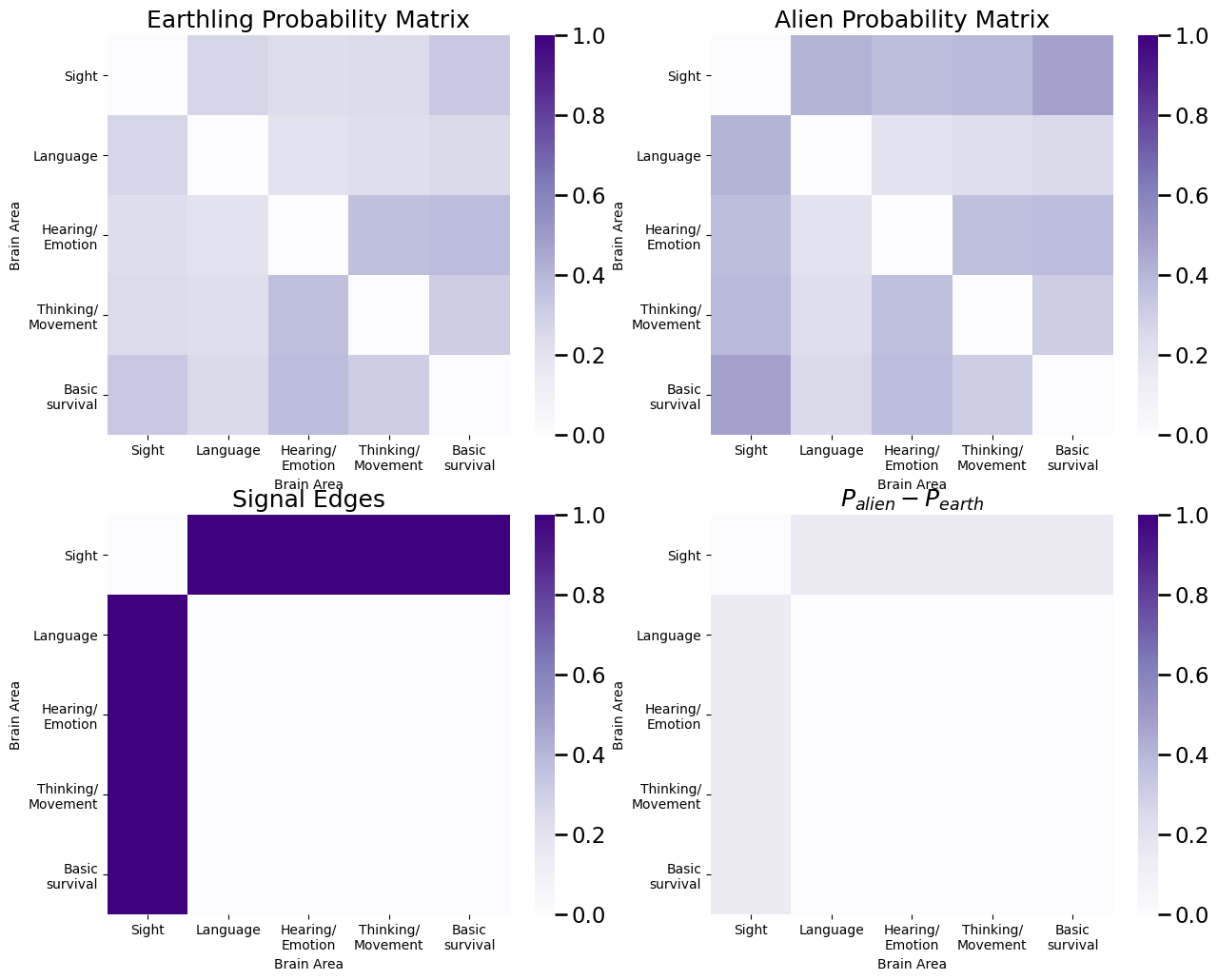
Next, we construct the probability matrices for each class. The probabilities for edges in which a node is in the sight area are higher for the aliens than the earthlings:

# the number of nodes
n = 5
# edge probabilities for earthlings are random
np.random.seed(12345)
P_hum = np.random.beta(size=n*n, a=3, b=8).reshape(n, n)
# networks are undirected, so make the probability matrix symmetric
P_hum = (P_hum + P_hum.T)/2
# networks are loopless, so remove the diagonal
P_hum = P_hum - np.diag(np.diag(P_hum))

# the names of each of the five nodes
nodenames = ["Sight", "Language", "Hearing/\nEmotion", "Thinking/\nMovement", "Basic\nsurvival"]
# the signal edges
E = np.array([[0,1,1,1,1], [1,0,0,0,0], [1,0,0,0,0], [1,0,0,0,0], [1,0,0,0,0]], dtype=bool)
P_alien = np.copy(P_hum)

# probabilities for signal edges are higher in aliens than earthlings
# 2/3 root function biases them towards 1, which is higher than
# whatever they are right now since they are between 0 and 1
P_alien[E] = np.power(P_alien[E], 2/3)

from matplotlib import pyplot as plt
import seaborn as sns

def plot_prob(X, title="", nodename="Brain Area", nodetix=[0.5, 1.5, 2.5, 3.5, 4.5],
             nodelabs=nodenames, ax=None, vmin=0, vmax=1):
    if (ax is None):
        fig, ax = plt.subplots(figsize=(8, 6))
    
    with sns.plotting_context("talk", font_scale=1):
        ax = sns.heatmap(X, cmap="Purples",
                        ax=ax, cbar_kws=dict(shrink=1), yticklabels=False,
                        xticklabels=False, vmin=vmin, vmax=vmax, annot=False)
        ax.set_title(title)
        cbar = ax.collections[0].colorbar
        ax.set(ylabel=nodename, xlabel=nodename)
        if (nodetix is not None) and (nodelabs is not None):
            ax.set_yticks(nodetix)
            ax.set_yticklabels(nodelabs)
            ax.set_xticks(nodetix)
            ax.set_xticklabels(nodelabs)
        cbar.ax.set_frame_on(True)
    return

fig, axs = plt.subplots(2,2, figsize=(15, 12))
plot_prob(P_hum, title="Earthling Probability Matrix", ax=axs[0,0])
plot_prob(P_alien, title="Alien Probability Matrix", ax=axs[0,1])
plot_prob(E, title="Signal Edges", ax=axs[1,0])
plot_prob(P_alien - P_hum, title="$P_{alien} - P_{earth}$", ax=axs[1,1])

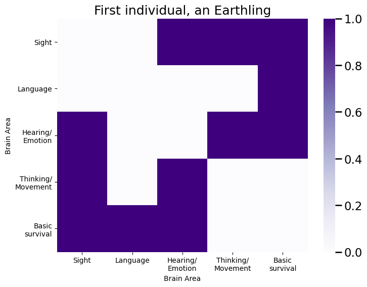
Finally, we use the class assignment vector \(\vec y\) to sample individual networks for each of the individuals. We plot an adjacency matrix for the first individual:

from graspologic.simulations import sample_edges

# arrange the probability matrices in a list
prob_mtxs = [P_alien, P_hum]
# initialize empty list for adjacency matrices
As = []
# generate seeds for reproducibility
seeds = np.random.randint(1, np.iinfo(np.int32).max, size=M)

for i, y in enumerate(yvec):
    # sample adjacency matrix for an individual of class y using the probability
    # matrix for that class
    np.random.seed(seeds[i])
    As.append(sample_edges(prob_mtxs[y - 1], directed=False, loops=False))

# stack the adjacency matrices for each individual such that node i is first dimension,
# node j is second dimension, and the individual index m is the third dimension
As = np.stack(As, axis=2)

from graspologic.plot import heatmap

fig, ax = plt.subplots(1,1, figsize=(8, 6));
plot_prob(As[:,:,0], title="First individual, an {}".format(classnames[yvec[0] - 1]), ax=ax);

The key ideas we want to capture in our classifier are as follows:

1. We want to only look at the edges which have a differing connection probability amongst our classes. This means that we only want to look at signal edges which are in the signal subnetwork, and we want to ignore edges which are not in the signal subnetwork. Edges which are not in the signal subnetwork are simply noise, since they have the same connection probability between the classes, and therefore are not useful for differentiating between the different classes.

2. We want to incorporate the structure of the network into the classifier. This means we want to use the fact that nodes are nodes, and that edges are connections between nodes, to determine how to classify networks as earthling or alien.

To begin, we will start by addressing aim 1. We need to find which edges are in the signal subnetwork. Stated another way, we need to estimate the signal subnetwork. What this requires is a way to identify which edges will best capture the difference between the classes in our network. Do we know anything which can do this? As it turns out, we can use Fisher’s exact test, something we learned about in the section on testing for differences between groups of edges in Section 6.2, to identify the signal subnetwork. In the next section on identifying significant vertices in Section 8.3, we will address the second point on using the structure of the network to further refine these potential signal edges.

8.2.1. Fisher’s Exact Test for Edge Importance

If you remember back to the coin flip example for the two-sample test with edge clusterings in Section 6.2.1.1.1, our setup was as follows. We had two coins, coin \(1\) and coin \(2\), and we wanted to test whether their probabilities of landing on heads were different. Our hypotheses were \(H_A: p_1 \neq p_2\), against the null hypothesis that \(H_0: p_1 = p_2\). We therefore had two random samples, the outcomes of ten coin flips from coin one and the outcomes of ten coin flips from coin two, meaning that our test of \(H_A\) against \(H_0\) fell into the two-sample testing regime. To address this, what we used was Fisher’s exact test, where we counted the number of times each coin landed on heads and tails, which we aggregated in a table:

	First coin	Second coin
Landed on heads	7	3
Landed on tails	3	7

As it turns out, we can adapt this test for our situation here too! For a single edge, what we want to do is test whether \(H_A: p_{ij}^{(alien)} \neq p_{ij}^{(earth)}\), against the null hypothesis that \(H_0: p_{ij}^{(alien)} = p_{ij}^{(earth)}\). The key property of Fisher’s exact test that makes it desirable for us is that, in a sense, when there is more evidence to support \(H_A\), the \(p\)-value will tend to be smaller, whereas when there is more evidence to support \(H_0\), the \(p\)-value will tend to be larger. We will exploit this feature in our design of a classifier for aliens versus earthlings. For each edge \((i, j)\), we will construct the following table:

	aliens	Earthlings
Edge \((i,j)\) exists	Number of aliens with edge \((i,j)\)	Number of earthlings with edge \((i,j)\)
Edge \((i,j)\) does not exist	Number of aliens without edge \((i,j)\)	Number of earthlings without edge \((i,j)\)

Which we can do in python as follows, for the edge from the sight area to the language area:

i = 1; j = 2  # (1,2) corresponds to the edge from sight to language

alien_edge = As[i-1,j-1,yvec == 1].sum()  # count the number of aliens with edge i,j
hum_edge = As[i-1,j-1,yvec == 2].sum()  # count the number of earthlings with edge i,j
alien_noedge = class_counts[1 - 1] - alien_edge  # count the number of aliens without edge i,j
hum_noedge = class_counts[2 - 1] - hum_edge  # count the number of earthlings without edge i,j

edge_tab = np.array([[alien_edge, hum_edge], [alien_noedge, hum_noedge]])  # arrange as in table shown above

print(edge_tab)

[[37. 24.]
 [50. 89.]]

Next, we compute the Fisher’s exact test \(p\)-value, using scipy:

from scipy.stats import fisher_exact

test_statistic, pval = fisher_exact(edge_tab)
print("p-value: {:.4f}".format(pval))

p-value: 0.0018

Note that since the edge \((i,j)\) that we chose above corresponded to the edge between the sight and language areas, we expect this edge to indicate a disparity between the aliens and the earthlings. Why is this?

Well, quite simply, by construction, this edge is a signal edge, which means that it carries real signal in differentiating a network from a earthling from a network of an alien. That the \(p\)-value is small tells us that we have evidence to reject the null hypothesis here in favor of the alternative hypothesis, that the edge from sight to language in fact shows a disparity between earthlings and aliens. Why is this a big deal?

Well, let’s see what happens if we were to compute this for a non-signal edge. Let’s arbitrarily choose the edge between the hearing/emotion and language areas, which corresponds to \(i=3\) (the hearing/emotion area) and \(j = 2\) (the language area):

i = 3; j = 2  # (3,2) corresponds to the edge from language to hearing

alien_edge = As[i-1,j-1,yvec == 1].sum()  # count the number of aliens with edge i,j
hum_edge = As[i-1,j-1,yvec == 2].sum()  # count the number of earthlings with edge i,j
alien_noedge = class_counts[1 - 1] - alien_edge  # count the number of aliens without edge i,j
hum_noedge = class_counts[2 - 1] - hum_edge  # count the number of earthlings without edge i,j

edge_tab = np.array([[alien_edge, hum_edge], [alien_noedge, hum_noedge]])  # arrange as in table shown above

test_statistic, pval = fisher_exact(edge_tab)
print("p-value: {:.4f}".format(pval))

p-value: 1.0000

Well, now this \(p\)-value happens to be a lot larger than the previous one we saw, now doesn’t it? Is this just by chance?

The answer is: no! The interpretation here is that we do not have evidence to reject the null hypothesis that the edge from language to hearing areas does not have a disparity between earthlings and aliens.

For signal edges, the \(p\)-value will, by construction, generally be smaller than the \(p\)-value in a non-signal edge. By generally, we mean that it will tend to be smaller (but not always!). We could certainly get samples of data where this is not the case, analogous to the idea that we could flip a fair coin (with equal probability of seeing heads and tails) 10 times and obtain all 10 flips being heads.

For this reason, we will use the Fisher’s exact test statistic to quantify how “important” an edge is for differentiating the two classes, or as an edge importance statistic. We will exploit this edge importance statistic as we build up our classifier further.

8.2.2. Using edge importances to estimate the signal subnetwork

We will use the Fisher’s exact \(p\)-value to develop an approach which allows us to properly estimate a signal subnetwork model. The key idea is this: if we were to use any one edge of the network, we would not really be able to predict whether someone is an earthling or an alien. The reason for this is that edges either exist, or not, so unless one of the class edge probabilities for a particular edge happens to be really low (near zero) and the other happens to be really high (near one), the only informative decision boundary we could construct would be to assign one class to the networks where that particular edge exists, or the other class to the networks where that particular edge does not exist. Even less interestingly, we could abitrarily say that every network is in a particular class, which is also not going to be a particularly interesting classifier.

Another thing we could do would be to use every edge in the network to develop a classifier, which also isn’t the best we could do. This is because if we use every edge in the classifier, we would have a lot of noise from the non-signal edges. This means that even though we might learn something from the signal edges, anything we learn is going to end up being diluted down by noise because we are including a lot of uninformative information in our classifier (the non-signal edges).

Rather, what we want to do is investigate to find the edges which are carrying all of the signal, and then isolate our downstream learning from information captured by those edges. This is because the signal edges carry all of the informative information about differentiating networks from one class to the other. This begs the question, how do we find the signal edges, and isolate them from the non-signal edges?

As we mentioned in the preceding subsection, as it happens, the Fisher’s exact test statistic is going to tend to be larger for edges in which there is actual signal (the edge probability is different for aliens and earthlings), and smaller when there is no signal (the edge probability is the same for aliens and earthlings). That is, if an edge is in the signal subnetwork, the Fisher’s exact test \(p\)-value is small, and if it is not in the signal subnetwork, the Fisher’s exact \(p\)-value is big. For this reason, what we end up doing is rank transforming the Fisher’s exact test \(p\)-values, and then pick an arbitrary number of the lowest ranking \(p\)-values to retain for classification.

We start by constructing a significance matrix, which is a collection of all of the Fisher’s exact test \(p\)-values for each edge:

fisher_mtx = np.zeros((n,n))
alien_idxs = yvec == 1  # the individuals who are aliens
hum_idxs = yvec == 2  # the individuals who are earthlings
# since the networks are undirected, only need to compute for upper triangle
for i in range(0, n):
    for j in range(i+1, n):
        alien_edgeij = As[i,j,alien_idxs].sum()
        hum_edgeij = As[i,j,hum_idxs].sum()
        table = np.array([[alien_edgeij, hum_edgeij],
                          [class_counts[0] - alien_edgeij, class_counts[1] - hum_edgeij]])
        fisher_mtx[i,j] = fisher_exact(table)[1]
fisher_mtx = fisher_mtx + fisher_mtx.T  # symmetrize

fig, ax = plt.subplots(1,1, figsize=(8, 6));
plot_prob(fisher_mtx, title="Fisher's exact $p$-values", vmax=fisher_mtx.max(), ax=ax)

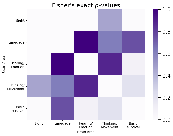
Notice that the edges with the highest Fisher’s exact test \(p\)-values in the significance matrix tend to be the edges with a node in the sight area, which are our signal edges. This is great news! Next, we rank the \(p\)-values in the significance matrix, from largest (a rank of 1) to smallest (the number of elements which are possible):

from scipy.stats import rankdata

sig_mtx = rankdata(np.max(fisher_mtx) - fisher_mtx).reshape(n,n)
sig_mtx = sig_mtx - np.diag(np.diag(sig_mtx))

fig, ax = plt.subplots(1,1, figsize=(8, 6));
plot_prob(sig_mtx, title="Ranked significance matrix", vmax=sig_mtx.max(), ax=ax)

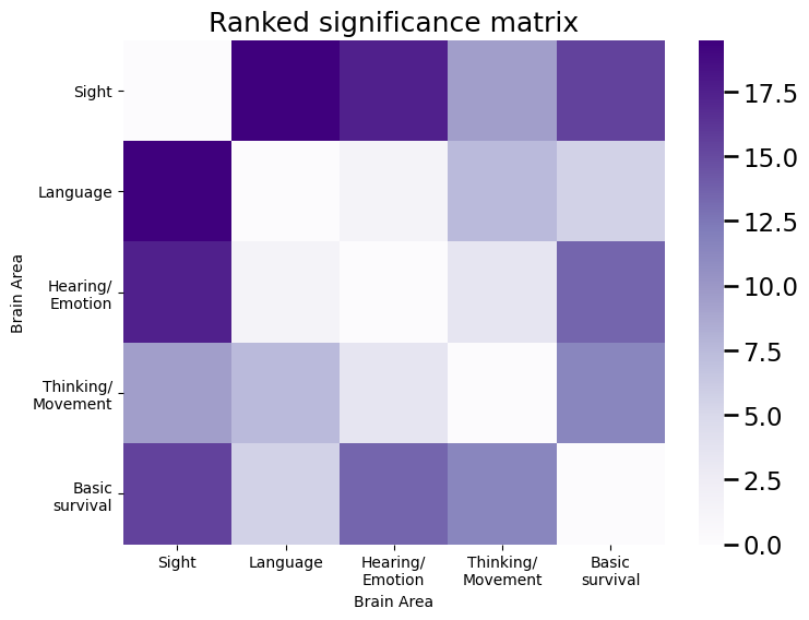
And the ranks tend to be larger for edges with a node in the sight area. Then, we select a number of edges (the size of the signal subnetwork) \(K\), and retain the top \(K\) edges, by their significance rankings. The top \(K\) edges by significance are an estimate of the signal subnetwork, \(\hat{\mathcal S}\).

We can implement everything we’ve learned so far in graspologic relatively easily, using the SignalSubgraph class:

from graspologic.subgraph import SignalSubgraph

K = 8  # the number of edges in the subgraph
sgest = SignalSubgraph()
sgest.fit_transform(As, labels=yvec - 1, constraints=K);

Next, we arrange this into a matrix so that we can look at the signal subnetwork we identified, and compare it to the true signal subnetwork:

sigsub = np.zeros((n,n))  # initialize empty matrix
sigsub[sgest.sigsub_] = 1

fig, axs = plt.subplots(1,2, figsize=(18, 6));
plot_prob(E, title="True Signal Subnetwork", ax=axs[0])
plot_prob(sigsub, title="Estimated Signal Subnetwork", ax=axs[1])

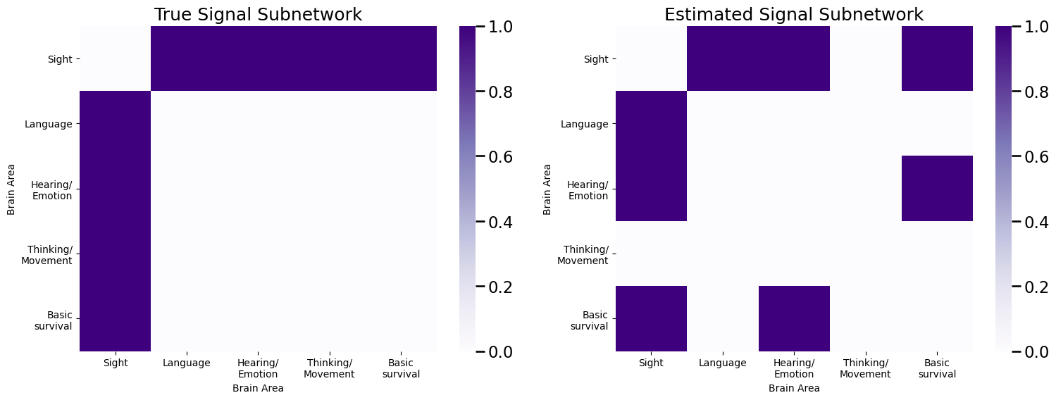
So our estimated signal subnetwork gets all of the edges correct except for the edge in the thinking/movement area.

A question you might be wondering concerns how exactly we chose the number of signal edges to include in our estimate of the signal subnetwork, \(\hat{\mathcal S}\). If we knew the number of edges in the signal subnetwork ahead of time, the choice would be easy: just choose \(K\) to be the number of edges in the signal subnetwork! In real data, however, this isn’t really going to be the case. For this reason, we will have to estimate \(K\) using \(\hat K\). To learn how to estimate \(K\), we first need to learn how to put what we’ve covered so far into a classifier, so read on!

8.2.3. Building a classifier using the estimated signal subnetwork

Finally, we can use the estimated signal subnetwork that we have constructed to devise a classifier. The objective of a classifier is to take new pieces of data (in this case, new networks), and assign them to the class which they are most likely from. How do we determine which class a network is most likely from?

At the moment, we have our estimate of the signal subnetwork, \(\hat{\mathcal S}\), and have a bunch of networks from one of two classes: alien (class 1) or alien (class 2). The edges of the network are binary, and we want to use the edges which are in the signal subnetwork to classify points as either alien or alien. A natural classifier choice for this situation is known as the Naive Bayes classifier. We have all the ingredients we need to construct a Naive Bayes classifier, so we’ll try to piece this together. For details on the intuition and background of this algorithm, check out the appendix section on the Naive Bayes classifier in Section 13.3 and the original paper [1].

8.2.3.1. Network classification

So, how do we actually use the estimated signal subnetwork \(\hat{\mathcal S}\) to classify new networks? Quite simply, we can just use sklearn’s BernoulliNB from sklearn, which is the Naive Bayes classifier for data where the features take values of \(0\) and \(1\) (such as our network). We need to reorganize our data a little bit to get it into the format we want. Our estimated signal subnetwork \(\hat{\mathcal S}\) is returned to us by graspologic in the format of a [2 x K] matrix, where \(K\) is the number of edges in the signal subnetwork. The first row is the row index of the entry of the signal subnetwork, and the second row is the column index of the entry in the signal subnetwork. We need to coerce this into an [M x K] matrix which we will call \(D\), where \(M\) is the total number of networks, and \(K\) is the number of edges in the signal subnetwork. Each entry of this matrix \(d_{mk}\) represents the adjacency value of the \(m^{th}\) individual for the \(k^{th}\) element of the signal subnetwork:

data = As[sgest.sigsub_[0], sgest.sigsub_[1],:].T

Next, we create a Naive Bayes classifier, and fit the classifier using the class vector \(\vec y\) for all of our samples:

from sklearn.naive_bayes import BernoulliNB

classifier = BernoulliNB()
# fit the classifier using the vector of classes for each sample
classifier.fit(data, yvec);

Let’s see how it does! We create \(200\) new networks, which are aliens or earthlings, and assess the performance using the classification accuracy:

Mtest = 200

# roll a 2-sided die 50 times, with probability 0.4 of landing on side 1 (alien) 
# and 0.6 of landing on side 2 (earthling)
np.random.seed(12345678)
class_countstest = np.random.multinomial(Mtest, pvals=[pi_alien, pi_hum])
print("Number of individuals who are aliens: {:d}".format(class_countstest[0]))
print("Number of individuals who are earthlings: {:d}".format(class_countstest[1]))

# create class assignment vector, and randomly reshuffle class labels for each individual
yvectest = np.array([1 for i in range(0, class_countstest[0])] + [2 for i in range(0, class_countstest[1])])
np.random.seed(12345678)
np.random.shuffle(yvectest)

Astest = []
np.random.seed(1234)
seeds = np.random.randint(1, np.iinfo(np.int32).max, size=Mtest)
for y in yvectest:
    # sample adjacency matrix for an individual of class y using the probability
    # matrix for that class
    Astest.append(sample_edges(prob_mtxs[y - 1], directed=False, loops=False))

# stack the adjacency matrices for each individual such that node i is first dimension,
# node j is second dimension, and the individual index m is the third dimension
Astest = np.stack(Astest, axis=2)

datatest = Astest[sgest.sigsub_[0], sgest.sigsub_[1],:].T

predictionstest = classifier.predict(datatest)

# classifier accuracy is the fraction of predictions that are correct
acc = np.mean(predictionstest == yvectest)
print("Classifier Accuracy: {:.3f}".format(acc))

Number of individuals who are aliens: 88
Number of individuals who are earthlings: 112
Classifier Accuracy: 0.630

Which means our classifier is right about \(60\%\) of the time. While the classifier tends to not perform too well on really small networks like the example data we are using here, we’d encourage you to try with bigger networks: it tends to do pretty well!

8.2.4. Selection of number of edges in signal subnetwork

If you remember above, we had a core question which was; how do we decide which number of edges to include in the estimated signal subnetwork?

Similar to other machine learning techniques, we use cross validation. Cross Validation is a procedure in which we split the dataset into a number of apprroximately equally sized splits (called folds), and then we train a machine learning model using a subset of the folds (the in-sample folds) and and test the trained model on the excluded subset of the folds (the out-of-sample folds).

So, how do we proceed for our dataset above? We begin by splitting the data into \(20\) folds, and then use \(20\)-fold cross validation to determine the accuracy of the resulting classifier when we include between \(4\) and \(20\) edges in the estimated signal subnetwork:

from sklearn.model_selection import KFold 
kf = KFold(n_splits=20, random_state=None)

xv_res = []
for k, (train_index, test_index) in enumerate(kf.split(range(0, M))):
    X_train, X_test = As[:,:,train_index], As[:,:,test_index]
    y_train = yvec[train_index]; y_test = yvec[test_index]
    
    for sgsz in np.arange(4, 21, step=2):
        # estimate ssg
        sgest = SignalSubgraph()
        sgest.fit_transform(X_train, labels=y_train - 1, constraints=int(sgsz));
        # train classifier
        data = X_train[sgest.sigsub_[0], sgest.sigsub_[1],:].T
        classifier = BernoulliNB()
        # fit the classifier using the vector of classes for each sample
        classifier.fit(data, y_train)
        
        datatest = X_test[sgest.sigsub_[0], sgest.sigsub_[1],:].T
        # evaluate performance on test fold        
        predictionstest = classifier.predict(datatest)

        # classifier accuracy is the fraction of predictions that are correct
        acc = np.mean(predictionstest == y_test)
        xv_res.append({"Fold": k+1, "K": sgsz, "Accuracy": acc})

import pandas as pd

df_res = pd.DataFrame(xv_res)

xv_acc = df_res.groupby(['K']).agg({"Accuracy": "mean"})

fig, ax = plt.subplots(1, 1, figsize=(8, 4))
sns.lineplot(x="K", y="Accuracy", data=xv_acc, ax=ax)

ax.set_xlabel("Number of Edges")
ax.set_ylabel("Average XV Accuracy")
ax.set_title("Determining optimal number of edges in signal subnetwork");

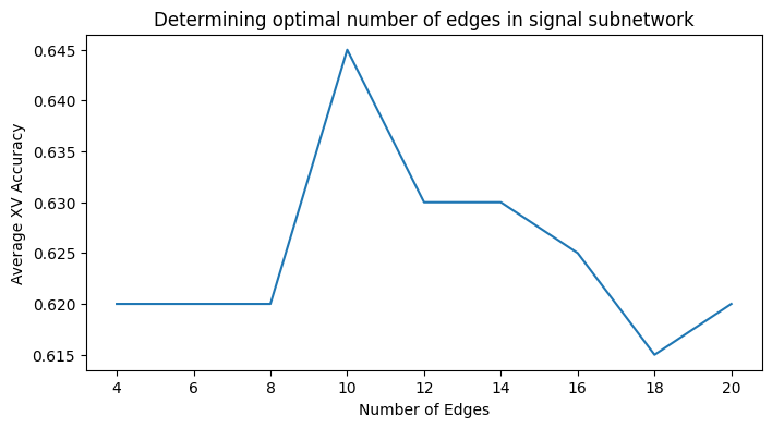
As we can see, the number of edges with the highest cross-validated accuracy is to include \(10\) edges in the signal subnetwork. When we produce an estimate of the signal subnetwork with \(10\) edges, we obtain:

Kopt = 10

sgest = SignalSubgraph()
sgest.fit_transform(As, labels=yvec - 1, constraints=Kopt);

sigsub = np.zeros((n,n))  # initialize empty matrix
sigsub[sgest.sigsub_] = 1

fig, axs = plt.subplots(1,2, figsize=(18, 6));
plot_prob(E, title="True Signal Subnetwork", ax=axs[0])
plot_prob(sigsub, title="Estimated Signal Subnetwork, $\hat K = 10$", ax=axs[1])

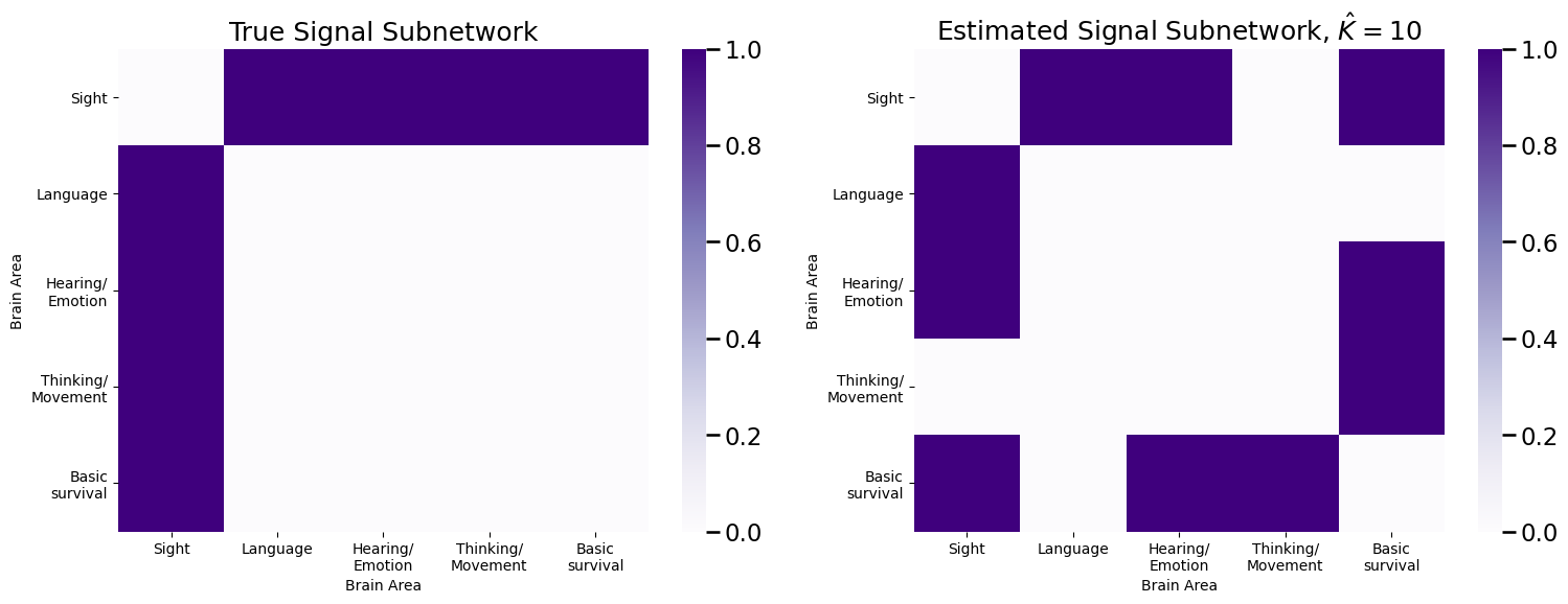
As we can see, we are now adding two additional edges which carry no signal. Can we be a little more intelligent with how we identify signal edges?

8.2.5. References

1

Joshua T. Vogelstein, William Gray Roncal, R. Jacob Vogelstein, and Carey E. Priebe. Graph classification using signal-subgraphs: applications in statistical connectomics. IEEE Trans. Pattern Anal. Mach. Intell., 35(7):1539–1551, July 2013. arXiv:23681985, doi:10.1109/TPAMI.2012.235.