Fisher’s method vs. min (after multiple comparison’s correction)#
Show code cell source
from pkg.utils import set_warnings

set_warnings()

import datetime
import time

import matplotlib.pyplot as plt
import numpy as np
import pandas as pd
import seaborn as sns
from myst_nb import glue as default_glue
from pkg.data import load_network_palette, load_node_palette, load_unmatched
from pkg.io import savefig
from pkg.plot import set_theme
from pkg.stats import stochastic_block_test
from graspologic.simulations import sbm
from tqdm import tqdm
import matplotlib.colors as colors
from scipy.stats import binom, combine_pvalues
from pkg.stats import binom_2samp
import matplotlib.colors as colors
from pathlib import Path


DISPLAY_FIGS = False

FILENAME = "compare_sbm_methods_sim"


def gluefig(name, fig, **kwargs):
    savefig(name, foldername=FILENAME, **kwargs)

    glue(name, fig, prefix="fig")

    if not DISPLAY_FIGS:
        plt.close()


def glue(name, var, prefix=None):
    savename = f"{FILENAME}-{name}"
    if prefix is not None:
        savename = prefix + ":" + savename
    default_glue(savename, var, display=False)


t0 = time.time()
set_theme()
rng = np.random.default_rng(8888)

network_palette, NETWORK_KEY = load_network_palette()
node_palette, NODE_KEY = load_node_palette()
fisher_color = sns.color_palette("Set2")[2]
min_color = sns.color_palette("Set2")[3]
method_palette = {"fisher": fisher_color, "min": min_color}

GROUP_KEY = "simple_group"

left_adj, left_nodes = load_unmatched(side="left")
right_adj, right_nodes = load_unmatched(side="right")

left_labels = left_nodes[GROUP_KEY].values
right_labels = right_nodes[GROUP_KEY].values
Show code cell source
stat, pvalue, misc = stochastic_block_test(
    left_adj,
    right_adj,
    labels1=left_labels,
    labels2=right_labels,
    method="fisher",
    combine_method="fisher",
)
Model for simulations (alternative)#
We have fit a stochastic block model to the left and right hemispheres. Say the probabilities of group-to-group connections on the left are stored in the matrix \(B\), so that \(B_{kl}\) is the probability of an edge from group \(k\) to \(l\).
Let \(\tilde{B}\) be a perturbed matrix of probabilities. We are interested in testing \(H_0: B = \tilde{B}\) vs. \(H_a: ... \neq ...\). To do so, we compare each \(H_0: B_{kl} = \tilde{B}_{kl}\) using Fisher’s exact test. This results in p-values for each \((k,l)\) comparison, \(\{p_{1,1}, p_{1,2}...p_{K,K}\}\).
Now, we still are after an overall test for the equality \(B = \tilde{B}\). Thus, we need a way to combine p-values \(\{p_{1,1}, p_{1,2}...p_{K,K}\}\) to get an overall p-value for our test comparing the stochastic block model probabilities. One way is Fisher’s method; another is to take the minimum p-value out of a collection of p-values which have been corrected for multiple comparisons (say, via Bonferroni or Holm-Bonferroni).
To compare how these two alternative methods of combining p-values work, we did the following simulation:
Let \(t\) be the number of probabilities to perturb.
Let \(\delta\) represent the strength of the perturbation (see model below).
For each trial:
Randomly select \(t\) probabilities without replacement from the elements of \(B\)
For each of these elements, \(\tilde{B}_{kl} = TN(B_{kl}, \delta B_{kl})\) where \(TN\) is a truncated normal distribution, such that probabilities don’t end up outside of [0, 1].
For each element not perturbed, \(\tilde{B}_{kl} = B_{kl}\)
Sample the number of edges from each block under each model. In other words, let \(m_{kl}\) be the number of edges in the \((k,l)\)-th block, and let \(n_k, n_l\) be the number of edges in the \(k\)-th and \(l\)-th blocks, respectively. Then, we have
\[m_{kl} \sim Binomial(n_k n_l, B_{kl})\]and likewise but with \(\tilde{B}_{kl}\) for \(\tilde{m}_{kl}\).
Run Fisher’s exact test to generate a \(p_{kl}\) for each \((k,l)\).
Run Fisher’s method for combining p-values, or take the minimum p-value after Bonferroni correction.
These trials were repeated for \(\delta \in \{0.1, 0.2, 0.3, 0.4, 0.5\}\) and \(t \in \{25, 50, 75, 100, 125\}\). For each \((\delta, t)\) we ran 100 replicates of the model/test above.
P-values under the null#
Show code cell source
B_base = misc["probabilities1"].values
inds = np.nonzero(B_base)
base_probs = B_base[inds]
n_possible_matrix = misc["possible1"].values
ns = n_possible_matrix[inds]

n_null_sims = 100

RERUN_NULL = False
save_path = Path(
    "/Users/bpedigo/JHU_code/bilateral/bilateral-connectome/results/"
    "outputs/compare_sbm_methods_sim/null_results.csv"
)

if RERUN_NULL:
    null_rows = []
    for sim in tqdm(range(n_null_sims)):
        base_samples = binom.rvs(ns, base_probs)
        perturb_samples = binom.rvs(ns, base_probs)

        # test on the new data
        def tester(cell):
            stat, pvalue = binom_2samp(
                base_samples[cell],
                ns[cell],
                perturb_samples[cell],
                ns[cell],
                null_odds=1,
                method="fisher",
            )
            return pvalue

        pvalue_collection = np.vectorize(tester)(np.arange(len(base_samples)))
        n_overall = len(pvalue_collection)
        pvalue_collection = pvalue_collection[~np.isnan(pvalue_collection)]
        n_tests = len(pvalue_collection)
        n_skipped = n_overall - n_tests

        row = {
            "sim": sim,
            "n_tests": n_tests,
            "n_skipped": n_skipped,
        }
        for method in ["fisher", "min"]:
            row = row.copy()
            if method == "min":
                overall_pvalue = min(pvalue_collection.min() * n_tests, 1)
                row["pvalue"] = overall_pvalue
            elif method == "fisher":
                stat, overall_pvalue = combine_pvalues(
                    pvalue_collection, method="fisher"
                )
                row["pvalue"] = overall_pvalue

            row["method"] = method
            null_rows.append(row)

    null_results = pd.DataFrame(null_rows)
    null_results.to_csv(save_path)
else:
    null_results = pd.read_csv(save_path, index_col=0)
Show code cell source
from giskard.plot import subuniformity_plot

fig, axs = plt.subplots(1, 2, figsize=(10, 5))
for i, method in enumerate(["fisher", "min"]):
    ax = axs[i]
    method_null_results = null_results[null_results["method"] == method]
    subuniformity_plot(
        method_null_results["pvalue"],
        ax=ax,
        color=method_palette[method],
        element="step",
    )
    ax.set_title(method.capitalize())

gluefig("null_distributions", fig)
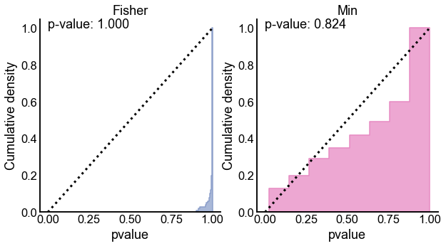
Distributions of p-values under the null for Fisher’s method (left) and the Min method (right) from a simulation with 100 resamples under the null. Dotted line indicates the CDF of a \(Uniform(0,1)\) random variable. The p-values in the upper left of each panel is for a 1-sample KS test, where the null is that the variable is distributed \(Uniform(0,1)\) against the alternative that its CDF is larger than that of a \(Uniform(0,1)\) random variable (i.e. that it is superuniform). Note that both methods appear empirically valid, but Fisher’s appears highly conservative.#
P-values under the alternative#
Show code cell source
n_sims = 100
n_perturb_range = np.linspace(0, 125, 6, dtype=int)[1:]
perturb_size_range = np.round(np.linspace(0, 0.5, 6), decimals=3)[1:]
print(f"Perturb sizes: {perturb_size_range}")
print(f"Perturb number range: {n_perturb_range}")
n_runs = n_sims * len(n_perturb_range) * len(perturb_size_range)
print(f"Number of runs: {n_runs}")
Perturb sizes: [0.1 0.2 0.3 0.4 0.5]
Perturb number range: [ 25  50  75 100 125]
Number of runs: 2500
Show code cell source
RERUN_SIM = False
save_path = Path(
    "/Users/bpedigo/JHU_code/bilateral/bilateral-connectome/results/"
    "outputs/compare_sbm_methods_sim/results.csv"
)

if RERUN_SIM:
    t0 = time.time()
    mean_itertimes = 0
    n_time_first = 5
    progress_steps = 0.05
    progress_counter = 0
    last_progress = -0.05
    simple_rows = []
    example_perturb_probs = {}
    for perturb_size in perturb_size_range:
        for n_perturb in n_perturb_range:
            for sim in range(n_sims):
                itertime = time.time()

                # just a way to track progress
                progress_counter += 1
                progress_prop = progress_counter / n_runs
                if progress_prop - progress_steps > last_progress:
                    print(f"{progress_prop:.2f}")
                    last_progress = progress_prop

                # choose some elements to perturb
                currtime = time.time()
                perturb_probs = base_probs.copy()
                choice_indices = rng.choice(
                    len(perturb_probs), size=n_perturb, replace=False
                )

                # pertub em
                for index in choice_indices:
                    prob = base_probs[index]

                    new_prob = -1
                    while new_prob <= 0 or new_prob >= 1:
                        new_prob = rng.normal(prob, scale=prob * perturb_size)

                    perturb_probs[index] = new_prob

                if sim == 0:
                    example_perturb_probs[(perturb_size, n_perturb)] = perturb_probs

                perturb_elapsed = time.time() - currtime

                # sample some new binomial data
                currtime = time.time()

                base_samples = binom.rvs(ns, base_probs)
                perturb_samples = binom.rvs(ns, perturb_probs)
                sample_elapsed = time.time() - currtime

                currtime = time.time()

                # test on the new data
                def tester(cell):
                    stat, pvalue = binom_2samp(
                        base_samples[cell],
                        ns[cell],
                        perturb_samples[cell],
                        ns[cell],
                        null_odds=1,
                        method="fisher",
                    )
                    return pvalue

                pvalue_collection = np.vectorize(tester)(np.arange(len(base_samples)))
                pvalue_collection = np.array(pvalue_collection)
                n_overall = len(pvalue_collection)
                pvalue_collection = pvalue_collection[~np.isnan(pvalue_collection)]
                n_tests = len(pvalue_collection)
                n_skipped = n_overall - n_tests
                test_elapsed = time.time() - currtime

                # combine pvalues
                currtime = time.time()
                row = {
                    "perturb_size": perturb_size,
                    "n_perturb": n_perturb,
                    "sim": sim,
                    "n_tests": n_tests,
                    "n_skipped": n_skipped,
                }
                for method in ["fisher", "min"]:
                    row = row.copy()
                    if method == "min":
                        overall_pvalue = min(pvalue_collection.min() * n_tests, 1)
                        row["pvalue"] = overall_pvalue
                    elif method == "fisher":
                        stat, overall_pvalue = combine_pvalues(
                            pvalue_collection, method="fisher"
                        )
                        row["pvalue"] = overall_pvalue

                    row["method"] = method
                    simple_rows.append(row)

                combine_elapsed = time.time() - currtime

                if progress_counter < n_time_first:
                    print("-----")
                    print(f"Perturb took {perturb_elapsed:0.3f}s")
                    print(f"Sample took {sample_elapsed:0.3f}s")
                    print(f"Test took {test_elapsed:0.3f}s")
                    print(f"Combine took {combine_elapsed:0.3f}s")
                    print("-----")
                    iter_elapsed = time.time() - itertime
                    mean_itertimes += iter_elapsed / n_time_first
                elif progress_counter == n_time_first:
                    projected_time = mean_itertimes * n_runs
                    projected_time = datetime.timedelta(seconds=projected_time)
                    print("---")
                    print(f"Projected time: {projected_time}")
                    print("---")

    total_elapsed = time.time() - t0

    print("Done!")
    print(f"Total experiment took: {datetime.timedelta(seconds=total_elapsed)}")
    results = pd.DataFrame(simple_rows)

    results.to_csv(save_path)
else:
    results = pd.read_csv(save_path, index_col=0)
Show code cell source
if RERUN_SIM:
    fig, axs = plt.subplots(
        len(perturb_size_range), len(n_perturb_range), figsize=(20, 20), sharey=True
    )

    for i, perturb_size in enumerate(perturb_size_range):
        for j, n_perturb in enumerate(n_perturb_range):
            ax = axs[i, j]
            perturb_probs = example_perturb_probs[(perturb_size, n_perturb)]
            mask = base_probs != perturb_probs
            show_base_probs = base_probs[mask]
            show_perturb_probs = perturb_probs[mask]
            sort_inds = np.argsort(-show_base_probs)
            show_base_probs = show_base_probs[sort_inds]
            show_perturb_probs = show_perturb_probs[sort_inds]

            sns.scatterplot(
                x=np.arange(len(show_base_probs)), y=show_perturb_probs, ax=ax, s=10
            )
            sns.lineplot(
                x=np.arange(len(show_base_probs)),
                y=show_base_probs,
                ax=ax,
                linewidth=1,
                zorder=-1,
                color="orange",
            )
            ax.set(xticks=[])

    ax.set(yscale="log")

    gluefig("example-perturbations", fig)
Show code cell source
fisher_results = results[results["method"] == "fisher"]
min_results = results[results["method"] == "min"]

fisher_means = fisher_results.groupby(["perturb_size", "n_perturb"]).mean()
min_means = min_results.groupby(["perturb_size", "n_perturb"]).mean()

mean_diffs = fisher_means["pvalue"] - min_means["pvalue"]
mean_diffs = mean_diffs.to_frame().reset_index()

mean_diffs_square = mean_diffs.pivot(
    index="perturb_size", columns="n_perturb", values="pvalue"
)

# v = np.max(np.abs(mean_diffs_square.values))

# fig, ax = plt.subplots(1, 1, figsize=(8, 8))
# sns.heatmap(
#     mean_diffs_square,
#     cmap="RdBu",
#     ax=ax,
#     yticklabels=perturb_size_range,
#     xticklabels=n_perturb_range,
#     square=True,
#     center=0,
#     vmin=-v,
#     vmax=v,
#     cbar_kws=dict(shrink=0.7),
# )
# ax.set(xlabel="Number of perturbed blocks", ylabel="Size of perturbation")
# cax = fig.axes[1]
# cax.text(4, 1, "Min more\nsensitive", transform=cax.transAxes, va="top")
# cax.text(4, 0, "Fisher more\nsensitive", transform=cax.transAxes, va="bottom")
# ax.set_title("(Fisher - Min) pvalues", fontsize="x-large")

# DISPLAY_FIGS = True
# gluefig("pvalue_diff_matrix", fig)
Show code cell source
fig, axs = plt.subplots(2, 3, figsize=(15, 10))


for i, perturb_size in enumerate(perturb_size_range):
    ax = axs.flat[i]
    plot_results = results[results["perturb_size"] == perturb_size]
    sns.lineplot(
        data=plot_results,
        x="n_perturb",
        y="pvalue",
        hue="method",
        style="method",
        palette=method_palette,
        ax=ax,
    )
    ax.set(yscale="log")
    ax.get_legend().remove()
    ax.axhline(0.05, color="dimgrey", linestyle=":")
    ax.axhline(0.005, color="dimgrey", linestyle="--")
    ax.set(ylabel="", xlabel="", title=f"{perturb_size}")

    ylim = ax.get_ylim()
    if ylim[0] < 1e-25:
        ax.set_ylim((1e-25, ylim[1]))

handles, labels = ax.get_legend_handles_labels()

ax.annotate(
    0.05,
    xy=(ax.get_xlim()[1], 0.05),
    xytext=(30, 10),
    textcoords="offset points",
    arrowprops=dict(arrowstyle="-"),
)
ax.annotate(
    0.005,
    xy=(ax.get_xlim()[1], 0.005),
    xytext=(30, -40),
    textcoords="offset points",
    arrowprops=dict(arrowstyle="-"),
)
axs.flat[-1].axis("off")

[ax.set(ylabel="p-value") for ax in axs[:, 0]]
[ax.set(xlabel="Number perturbed") for ax in axs[1, :]]
axs[0, -1].set(xlabel="Number perturbed")

axs[0, 0].set_title(f"Perturbation size = {perturb_size_range[0]}")

for i, label in enumerate(labels):
    labels[i] = label.capitalize()
axs.flat[-1].legend(handles=handles, labels=labels, title="Method")

gluefig("perturbation_pvalues_lineplots", fig)
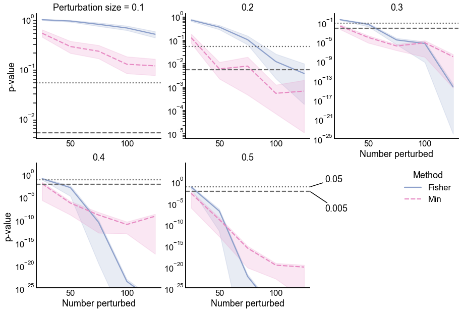
p-values under the alternative for two different methods for combining p-values: Fisher’s method (performed on the uncorrected p-values) and simply taking the minimum p-value after Bonferroni correction (here, called Min). The alternative is specified by changing the number of probabilities which are perturbed (x-axis in each panel) as well as the size of the perturbations which are done to each probability (panels show increasing perturbation size). Dotted and dashed lines indicate significance thresholds for \(\alpha = \{0.05, 0.005\}\), respectively. Note that in this simulation, even for large numbers of small perturbations (i.e. upper left panel), the Min method has smaller p-values. Fisher’s method displays smaller p-values than Min only when there are many (>50) large perturbations, but by this point both methods yield extremely small p-values.#
Power under the alternative#
Show code cell source
alpha = 0.05
results["detected"] = 0
results.loc[results[(results["pvalue"] < alpha)].index, "detected"] = 1
Show code cell source
fisher_results = results[results["method"] == "fisher"]
min_results = results[results["method"] == "min"]

fisher_means = fisher_results.groupby(["perturb_size", "n_perturb"]).mean()
min_means = min_results.groupby(["perturb_size", "n_perturb"]).mean()

fisher_power_square = fisher_means.reset_index().pivot(
    index="perturb_size", columns="n_perturb", values="detected"
)
min_power_square = min_means.reset_index().pivot(
    index="perturb_size", columns="n_perturb", values="detected"
)

mean_diffs = fisher_means["detected"] / min_means["detected"]

mean_diffs = mean_diffs.to_frame().reset_index()

ratios_square = mean_diffs.pivot(
    index="perturb_size", columns="n_perturb", values="detected"
)

v = np.max(np.abs(mean_diffs_square.values))

# fig, axs = plt.subplots(1, 3, figsize=(12, 4), sharex=True, sharey=True)
from matplotlib.transforms import Bbox

set_theme(font_scale=1.5)
# set up plot
pad = 0.5
width_ratios = [1, pad * 1.2, 10, pad, 10, 1.3 * pad, 10, 1]
fig, axs = plt.subplots(
    1,
    len(width_ratios),
    figsize=(30, 10),
    gridspec_kw=dict(
        width_ratios=width_ratios,
    ),
)
fisher_col = 2
min_col = 4
ratio_col = 6


def shrink_axis(ax, scale=0.7):
    pos = ax.get_position()
    mid = (pos.ymax + pos.ymin) / 2
    height = pos.ymax - pos.ymin
    new_pos = Bbox(
        [
            [pos.xmin, mid - scale * 0.5 * height],
            [pos.xmax, mid + scale * 0.5 * height],
        ]
    )
    ax.set_position(new_pos)


def power_heatmap(
    data, ax=None, center=0, vmin=0, vmax=1, cmap="RdBu_r", cbar=False, **kwargs
):
    out = sns.heatmap(
        data,
        ax=ax,
        yticklabels=perturb_size_range,
        xticklabels=n_perturb_range,
        square=True,
        center=center,
        vmin=vmin,
        vmax=vmax,
        cbar_kws=dict(shrink=0.7),
        cbar=cbar,
        cmap=cmap,
        **kwargs,
    )
    ax.invert_yaxis()
    return out


ax = axs[fisher_col]
im = power_heatmap(fisher_power_square, ax=ax)
ax.set_title("Fisher's method", fontsize="large")

ax = axs[0]
shrink_axis(ax, scale=0.5)
_ = fig.colorbar(
    im.get_children()[0],
    cax=ax,
    fraction=1,
    shrink=1,
    ticklocation="left",
)
ax.set_title("Power\n" + r"($\alpha=0.05$)", pad=25)

ax = axs[min_col]
power_heatmap(min_power_square, ax=ax)
ax.set_title("Min method", fontsize="large")
ax.set(yticks=[])

pal = sns.diverging_palette(145, 300, s=60, as_cmap=True)

ax = axs[ratio_col]
im = power_heatmap(np.log10(ratios_square), ax=ax, vmin=-2, vmax=2, center=0, cmap=pal)
# ax.set_title(r'$log_10(\frac{\text{Power}_{Fisher}}{\text{Power}_{Min}})$')
# ax.set_title(
#     r"$log_{10}($Fisher power$)$" + "\n" + r" - $log_{10}($Min power$)$",
#     fontsize="large",
# )
ax.set(yticks=[])

ax = axs[-1]
shrink_axis(ax, scale=0.5)
_ = fig.colorbar(
    im.get_children()[0],
    cax=ax,
    fraction=1,
    shrink=1,
    ticklocation="right",
)
ax.text(2, 1, "Fisher more\nsensitive", transform=ax.transAxes, va="top")
ax.text(2, 0.5, "Equal power", transform=ax.transAxes, va="center")
ax.text(2, 0, "Min more\nsensitive", transform=ax.transAxes, va="bottom")
ax.set_title("Log10\npower\nratio", pad=20)

# remove dummy axes
for i in range(len(width_ratios)):
    if not axs[i].has_data():
        axs[i].set_visible(False)

xlabel = r"# perturbed blocks $\rightarrow$"
ylabel = r"Perturbation size $\rightarrow$"
axs[fisher_col].set(
    xlabel=xlabel,
    ylabel=ylabel,
)
axs[min_col].set(xlabel=xlabel, ylabel="")
axs[ratio_col].set(xlabel=xlabel, ylabel="")

fig.text(0.09, 0.86, "A)", fontweight="bold", fontsize=50)
fig.text(0.64, 0.86, "B)", fontweight="bold", fontsize=50)
gluefig("relative_power", fig)
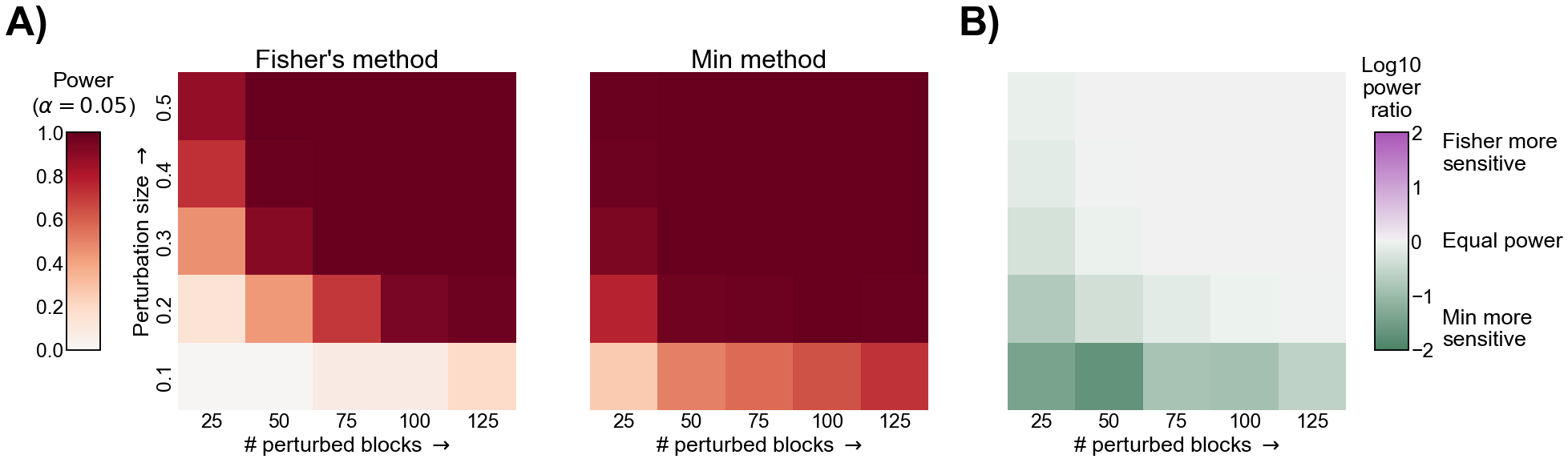
Comparison of power for Fisher’s and the Min method. A) The power under the alternative described in the text for both Fisher’s method and the Min method. In both heatmaps, the x-axis represents an increasing number of blocks which are perturbed, and the y-axis represents an increasing magnitude for each perturbation. B) The log of the ratio of powers (Fisher’s / Min) for each alternative. Note that positive (purple) values would represent that Fisher’s is more powerful, and negative (green) represent that the Min method is more powerful. Notice that the Min method appears to have more power for subtler (fewer or smaller perturbations) alternatives, and nearly equal power for more obvious alternatives.#