An exact test for non-unity null odds ratios

Show code cell source Hide code cell source

from pkg.utils import set_warnings

set_warnings()

import matplotlib.pyplot as plt
import numpy as np
import pandas as pd
import seaborn as sns
from giskard.plot import set_theme, subuniformity_plot
from matplotlib.figure import Figure
from myst_nb import glue
from scipy.stats import binom, fisher_exact
from pkg.stats import fisher_exact_nonunity

set_theme()


def my_glue(name, variable):
    glue(name, variable, display=False)
    if isinstance(variable, Figure):
        plt.close()

Simulation setup

Here, we investigate the performance of this test on simulated independent binomials. The model we use is as follows:

Let

\[X \sim Binomial(m_x, p_x)\]

independently,

\[Y \sim Binomial(m_y, p_y)\]

Fix \(m_x = \) 1000, \(m_y = \) 2000, \(p_y = \) 0.01.

Let \(p_x = \omega p_y\), where \(\omega\) is some positive real number, not not necessarily equal to 1, such that \(p_x \in (0, 1)\).

Show code cell source Hide code cell source

m_x = 1000
my_glue("m_x", m_x)
m_y = 2000
my_glue("m_y", m_y)

upper_omegas = np.linspace(1, 4, 7)
lower_omegas = 1 / upper_omegas
lower_omegas = lower_omegas[1:]
omegas = np.sort(np.concatenate((upper_omegas, lower_omegas)))
my_glue("upper_omega", max(omegas))
my_glue("lower_omega", min(omegas))


p_y = 0.01
my_glue("p_y", p_y)

n_sims = 200
my_glue("n_sims", n_sims)

alternative = "two-sided"

Experiment

Below, we’ll sample from the model described above, varying \(\omega\) from 0.25 to 4.0. For each value of \(\omega\), we’ll draw 200 samples of \((x,y)\) from the model described above. For each draw, we’ll test the following two hypotheses:

\[H_0: p_x = p_y \quad H_A: p_x \neq p_y\]

using Fisher’s exact test, and

\[H_0: p_x = \omega_0 p_y \quad H_A: p_x \neq \omega_0 p_y\]

using a modified version of Fisher’s exact test, which uses Fisher’s noncentral hypergeometric distribution as the null distribution. Note that we can re-write this null as

\[H_0: \frac{p_x}{p_y} = \omega_0\]

to easily see that this is a test for a posited odds ratio \(\omega_0\). For this experiment, we set \(\omega_0 = \omega\) - in other words, we assume the true odds ratio is known.

Below, we’ll call the first hypothesis test FE (Fisher’s Exact), and the second NUFE (Non-unity Fisher’s Exact).

Show code cell source Hide code cell source

# definitions following https://en.wikipedia.org/wiki/Fisher%27s_noncentral_hypergeometric_distribution

rows = []
for omega in omegas:
    # params
    p_x = omega * p_y
    omega_x = p_x / (1 - p_x)
    omega_y = p_y / (1 - p_y)

    for sim in range(n_sims):
        # sample
        x = binom.rvs(m_x, p_x)
        y = binom.rvs(m_y, p_y)
        n = x + y

        table = np.array([[x, m_x - x], [y, m_y - y]])
        _, vanilla_pvalue = fisher_exact(table, alternative=alternative)
        _, nu_pvalue = fisher_exact_nonunity(
            table, alternative=alternative, null_odds=omega
        )

        rows.append(
            {
                "method": "FE",
                "omega": omega,
                "pvalue": vanilla_pvalue,
                "sim": sim,
            }
        )

        rows.append({"method": "NUFE", "omega": omega, "pvalue": nu_pvalue, "sim": sim})


results = pd.DataFrame(rows)

Results

Show code cell source Hide code cell source

colors = sns.color_palette()
palette = {"FE": colors[0], "NUFE": colors[1]}

fig, ax = plt.subplots(1, 1, figsize=(8, 6))

sns.lineplot(data=results, x="omega", y="pvalue", hue="method", ax=ax, palette=palette)
ax.axvline(1, color="darkred", linestyle="--")
ax.set(ylabel="p-value", xlabel=r"$\omega$")

my_glue("fig_mean_pvalue_by_omega", fig)

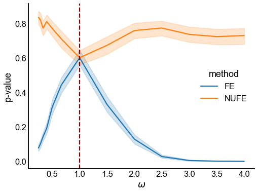
Fig. 10 Plot of mean p-values by the true odds ratio \(\omega\). Each point in the lineplot denotes the mean over 200 trials, and the shaded region denotes 95% bootstrap CI estimates. Fisher’s Exact test (FE) tends to reject for non-unity odds ratios, while the modified, non-unity Fisher’s exact test (NUFE) does not. Note that NUFE is testing the null hypothesis that the odds ratio (\(\omega_0\)) is equal to the true odds ratio in the simulation (\(\omega\)).

Show code cell source Hide code cell source

def plot_select_pvalues(method, omega, ax):

    subuniformity_plot(
        results[(results["method"] == method) & (results["omega"] == omega)][
            "pvalue"
        ].values,
        color=palette[method],
        ax=ax,
    )
    ax.set(title=r"$\omega = $" + f"{omega}, method = {method}", xlabel="p-value")


fig, axs = plt.subplots(1, 2, figsize=(12, 6))
plot_select_pvalues(method="FE", omega=1, ax=axs[0])
plot_select_pvalues(method="NUFE", omega=1, ax=axs[1])

my_glue("fig_pvalue_dist_omega_1", fig)

fig, axs = plt.subplots(1, 2, figsize=(12, 6))
plot_select_pvalues(method="FE", omega=3, ax=axs[0])
plot_select_pvalues(method="NUFE", omega=3, ax=axs[1])

my_glue("fig_pvalue_dist_omega_3", fig)

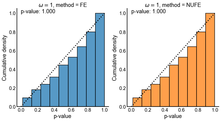
Fig. 11 Cumulative distribution of p-values for both tests when the true odds ratio \(\omega = 1\). Dashed line denotes the cumulative distribution function for a \(Uniform(0,1)\) random variable. p-value in upper left is for a one-sided KS-test that for the null that the distribution is stochastically smaller than a \(Uniform(0,1)\) random variable. Note that both tests appear to have uniform p-values in the case where the null that both tests are concerned with is true.

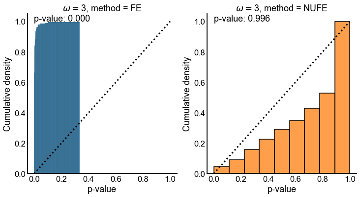
Fig. 12 Cumulative distribution of p-values for both tests when the true odds ratio \(\omega = 3\). Dashed line denotes the cumulative distribution function for a \(Uniform(0,1)\) random variable. p-value in upper left is for a one-sided KS-test that for the null that the distribution is stochastically smaller than a \(Uniform(0,1)\) random variable. When \(\omega = 3\), the null that FE is testing is indeed false, so it makes sense that we see yield many small p-values. However, for \(NUFE\), \(H_0\) is true, as we specified that \(\omega_0 = \omega\). NUFE remains valid in this case as the p-values appear stochastically smaller than a \(Uniform(0,1)\) random variable.