A group-based test#
Show code cell source
from pkg.utils import set_warnings

set_warnings()

import datetime
import time

import matplotlib.pyplot as plt
import numpy as np
import pandas as pd
import seaborn as sns
from myst_nb import glue as default_glue
from pkg.data import load_matched, load_network_palette, load_node_palette
from pkg.io import savefig
from pkg.perturb import remove_edges
from pkg.plot import set_theme
from pkg.stats import stochastic_block_test_paired
from seaborn.utils import relative_luminance

DISPLAY_FIGS = False
FILENAME = "sbm_matched_test"

rng = np.random.default_rng(8888)


def gluefig(name, fig, **kwargs):
    savefig(name, foldername=FILENAME, **kwargs)

    glue(name, fig, prefix="fig")

    if not DISPLAY_FIGS:
        plt.close()


def glue(name, var, prefix=None):
    savename = f"{FILENAME}-{name}"
    if prefix is not None:
        savename = prefix + ":" + savename
    default_glue(savename, var, display=False)


t0 = time.time()
set_theme(font_scale=1.25)

network_palette, NETWORK_KEY = load_network_palette()
node_palette, NODE_KEY = load_node_palette()

left_adj, left_nodes = load_matched("left")
right_adj, right_nodes = load_matched("right")
A test based on group connection probabilities#
Run the test#
Show code cell source
# TODO double check that all simple groups are the same
stat, pvalue, misc = stochastic_block_test_paired(
    left_adj, right_adj, labels=left_nodes["simple_group"]
)
glue("uncorrected_pvalue", pvalue)
Plot the p-values for the individual comparisons#
Show code cell source
uncorrected_pvalues = misc["uncorrected_pvalues"]
n_tests = misc["n_tests"]
K = uncorrected_pvalues.shape[0]
alpha = 0.05
hb_thresh = alpha / n_tests
index = uncorrected_pvalues.index

fig, ax = plt.subplots(1, 1, figsize=(8, 8))
# colors = im.get_children()[0].get_facecolors()
significant = uncorrected_pvalues < hb_thresh
pvalue_vmin = np.nanmin(np.log10(uncorrected_pvalues.values))
# annot = np.full((K, K), "")
# annot[(B1.values == 0) & (B2.values == 0)] = "B"
# annot[(B1.values == 0) & (B2.values != 0)] = "L"
# annot[(B1.values != 0) & (B2.values == 0)] = "R"

plot_pvalues = np.log10(uncorrected_pvalues)
plot_pvalues[np.isnan(plot_pvalues)] = 0
im = sns.heatmap(
    plot_pvalues,
    ax=ax,
    # annot=annot,
    cmap="RdBu",
    center=0,
    square=True,
    cbar=True,
    vmin=pvalue_vmin,
    cbar_kws=dict(shrink=0.6),
)
ax.set(ylabel="", xlabel="Target group")
ax.set(xticks=np.arange(K) + 0.5, xticklabels=index)
ax.set(yticks=np.arange(K) + 0.5, yticklabels=index)
ax.set_title(r"$log_{10}($p-value$)$", fontsize="xx-large")

colors = im.get_children()[0].get_facecolors()
significant = uncorrected_pvalues < hb_thresh

# NOTE: the x's looked bad so I did this super hacky thing...
pad = 0.2
for idx, (is_significant, color) in enumerate(zip(significant.values.ravel(), colors)):
    if is_significant:
        i, j = np.unravel_index(idx, (K, K))
        # REF: seaborn heatmap
        lum = relative_luminance(color)
        text_color = ".15" if lum > 0.408 else "w"

        xs = [j + pad, j + 1 - pad]
        ys = [i + pad, i + 1 - pad]
        ax.plot(xs, ys, color=text_color, linewidth=4)
        xs = [j + 1 - pad, j + pad]
        ys = [i + pad, i + 1 - pad]
        ax.plot(xs, ys, color=text_color, linewidth=4)

gluefig("uncorrected_pvalues", fig)
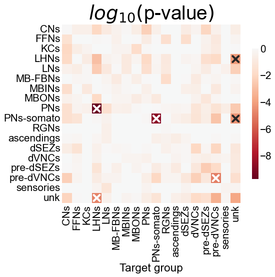
Fig. 14 The p-values for each hypothesis test between individual elements of the block probability matrices. Each comparison was done by McNemar’s test, which treats each potential edge as a potential, and examines whether the number of disagreeing edges between the left and right is likely to be observed by chance. “X” denotes a significant p-value after Bonferroni-Holm correction, with \(\alpha=0.05\). These individual p-values were combined using Fisher’s method, resulting in an overall p-value of 1.15e-10.#
Correcting for a global difference in density#
Compute the density correction#
Show code cell source
n_edges_left = np.count_nonzero(left_adj)
n_edges_right = np.count_nonzero(right_adj)
n_left = left_adj.shape[0]
n_right = right_adj.shape[0]
density_left = n_edges_left / (n_left ** 2)
density_right = n_edges_right / (n_right ** 2)

n_remove = int((density_right - density_left) * (n_right ** 2))

glue("density_left", density_left)
glue("density_right", density_right)
glue("n_remove", n_remove)
Subsample edges on the right hemisphere to set the densities the same#
Show code cell source
rows = []
n_resamples = 25
glue("n_resamples", n_resamples)
for i in range(n_resamples):
    subsampled_right_adj = remove_edges(
        right_adj, effect_size=n_remove, random_seed=rng
    )
    stat, pvalue, misc = stochastic_block_test_paired(
        left_adj, subsampled_right_adj, labels=left_nodes["simple_group"]
    )
    rows.append({"stat": stat, "pvalue": pvalue, "misc": misc, "resample": i})

resample_results = pd.DataFrame(rows)
Plot the p-values for the corrected tests#
Show code cell source
fig, ax = plt.subplots(1, 1, figsize=(8, 6))
sns.histplot(data=resample_results, x="pvalue", ax=ax)
ax.set(xlabel="p-value", ylabel="", yticks=[])
ax.spines["left"].set_visible(False)

mean_resample_pvalue = np.mean(resample_results["pvalue"])
median_resample_pvalue = np.median(resample_results["pvalue"])

gluefig("pvalues_corrected", fig)
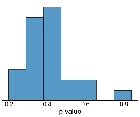
Fig. 15 Histogram of p-values after a correction for network density. For the observed networks the left hemisphere has a density of 0.0191, and the right hemisphere has a density of 0.0208. Here, we randomly removed exactly edges from the right hemisphere network, which makes the density of the right network match that of the left hemisphere network. Then, we re-ran the stochastic block model testing procedure from Figure 14. This entire process was repeated times. The histogram above shows the distribution of p-values for the overall test. Note that the p-values are no longer small, indicating that with this density correction, we now failed to reject our null hypothesis of bilateral symmetry (after density correction) under the stochastic block model.#
Show code cell source
elapsed = time.time() - t0
delta = datetime.timedelta(seconds=elapsed)
print(f"Script took {delta}")
print(f"Completed at {datetime.datetime.now()}")
Script took 0:00:10.066310
Completed at 2021-11-11 08:54:25.067608