Comparing methods for SBM testing#
Show code cell source
import csv
import datetime
import time
from pathlib import Path

import matplotlib.pyplot as plt
import numpy as np
import pandas as pd
import seaborn as sns
from matplotlib.transforms import Bbox
from pkg.data import load_network_palette, load_unmatched
from pkg.io import FIG_PATH, get_environment_variables
from pkg.io import glue as default_glue
from pkg.io import savefig
from pkg.plot import SmartSVG, set_theme, subuniformity_plot, svg_to_pdf
from pkg.stats import binom_2samp, stochastic_block_test
from scipy.stats import binom, combine_pvalues
from statsmodels.stats.contingency_tables import StratifiedTable
from svgutils.compose import Figure, Panel, Text
from tqdm.autonotebook import tqdm


_, RERUN_SIMS, DISPLAY_FIGS = get_environment_variables()


FILENAME = "revamp_sbm_methods_sim"

FIG_PATH = FIG_PATH / FILENAME


def glue(name, var, **kwargs):
    default_glue(name, var, FILENAME, **kwargs)


def gluefig(name, fig, **kwargs):
    savefig(name, foldername=FILENAME, **kwargs)

    glue(name, fig, figure=True)

    if not DISPLAY_FIGS:
        plt.close()


t0 = time.time()
set_theme()
rng = np.random.default_rng(8888)

network_palette, NETWORK_KEY = load_network_palette()
fisher_color = sns.color_palette("Set2")[2]
min_color = sns.color_palette("Set2")[3]
eric_color = sns.color_palette("Set2")[4]

GROUP_KEY = "simple_group"

left_adj, left_nodes = load_unmatched(side="left")
right_adj, right_nodes = load_unmatched(side="right")

left_labels = left_nodes[GROUP_KEY].values
right_labels = right_nodes[GROUP_KEY].values
Environment variables:
   RESAVE_DATA: true
   RERUN_SIMS: true
   DISPLAY_FIGS: False
Show code cell source
stat, pvalue, misc = stochastic_block_test(
    left_adj,
    right_adj,
    labels1=left_labels,
    labels2=right_labels,
    method="fisher",
    combine_method="fisher",
)
Model for simulations (alternative)#
We have fit a stochastic block model to the left and right hemispheres. Say the probabilities of group-to-group connections on the left are stored in the matrix \(B\), so that \(B_{kl}\) is the probability of an edge from group \(k\) to \(l\).
Let \(\tilde{B}\) be a perturbed matrix of probabilities. We are interested in testing \(H_0: B = \tilde{B}\) vs. \(H_a: ... \neq ...\). To do so, we compare each \(H_0: B_{kl} = \tilde{B}_{kl}\) using Fisher’s exact test. This results in p-values for each \((k,l)\) comparison, \(\{p_{1,1}, p_{1,2}...p_{K,K}\}\).
Now, we still are after an overall test for the equality \(B = \tilde{B}\). Thus, we need a way to combine p-values \(\{p_{1,1}, p_{1,2}...p_{K,K}\}\) to get an overall p-value for our test comparing the stochastic block model probabilities. One way is Fisher’s method; another is Tippett’s method.
To compare how these two alternative methods of combining p-values work, we did the following simulation:
Let \(t\) be the number of probabilities to perturb.
Let \(\delta\) represent the strength of the perturbation (see model below).
For each trial:
Randomly select \(t\) probabilities without replacement from the elements of \(B\)
For each of these elements, \(\tilde{B}_{kl} = TN(B_{kl}, \delta B_{kl})\) where \(TN\) is a truncated normal distribution, such that probabilities don’t end up outside of [0, 1].
For each element not perturbed, \(\tilde{B}_{kl} = B_{kl}\)
Sample the number of edges from each block under each model. In other words, let \(m_{kl}\) be the number of edges in the \((k,l)\)-th block, and let \(n_k, n_l\) be the number of edges in the \(k\)-th and \(l\)-th blocks, respectively. Then, we have
\[m_{kl} \sim Binomial(n_k n_l, B_{kl})\]and likewise but with \(\tilde{B}_{kl}\) for \(\tilde{m}_{kl}\).
Run Fisher’s exact test to generate a \(p_{kl}\) for each \((k,l)\).
Run Fisher’s or Tippett’s method for combining p-values
These trials were repeated for \(\delta \in \{0.1, 0.2, 0.3, 0.4, 0.5\}\) and \(t \in \{25, 50, 75, 100, 125\}\). For each \((\delta, t)\) we ran 100 replicates of the model/test above.
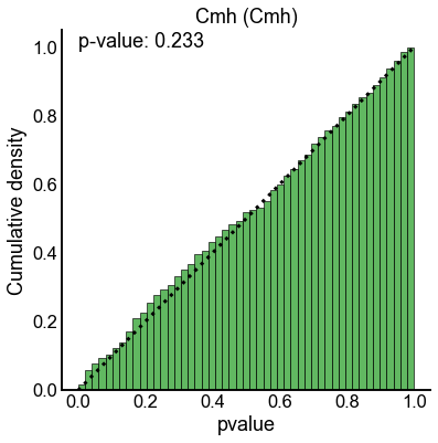
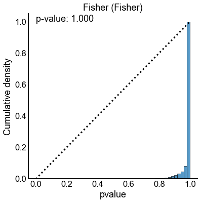
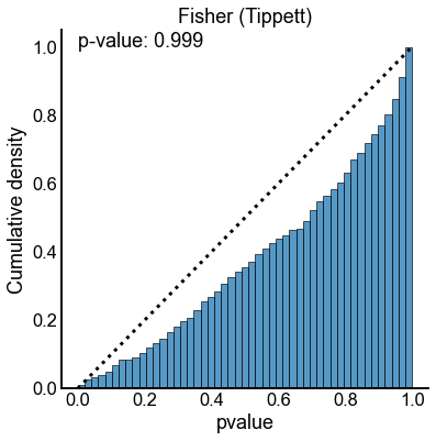
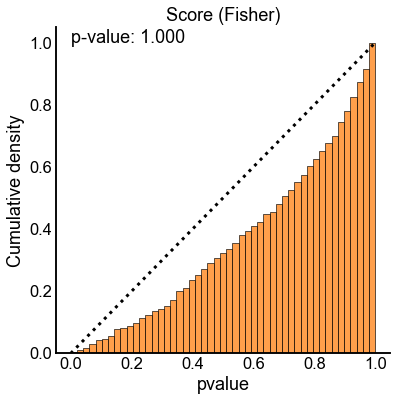
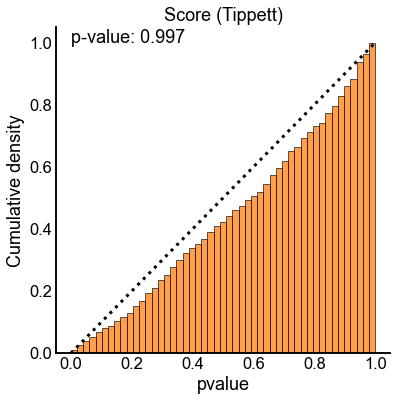
P-values under the null#
P-values under the alternative#
Show code cell source
# def random_shift_pvalues(pvalues, rng=None):
#     pvalues = np.sort(pvalues)  # already makes a copy
#     diffs = list(pvalues[1:] - pvalues[:-1])
#     if rng is None:
#         rng = np.random.default_rng()
#     uniform_samples = rng.uniform(size=len(diffs))
#     moves = uniform_samples * diffs
#     pvalues[1:] = pvalues[1:] - moves
#     return pvalues


# def my_combine_pvalues(pvalues, method="fisher", pad_high=0, n_resamples=100):
#     pvalues = np.array(pvalues)
#     # some methods use log(1 - pvalue) as part of the test statistic - thus when pvalue
#     # is exactly 1 (which is possible for Fisher's exact test) we get an underfined
#     # answer.
#     if pad_high > 0:
#         upper_lim = 1 - pad_high
#         pvalues[pvalues >= upper_lim] = upper_lim

#     scipy_methods = ["fisher", "pearson", "tippett", "stouffer", "mudholkar_george"]

#     if method == "fisher-discrete-random":
#         stat = 0
#         pvalue = 0
#         shifted_pvalues = []
#         for i in range(n_resamples):
#             shifted_pvalues = random_shift_pvalues(pvalues)
#             curr_stat, curr_pvalue = scipy_combine_pvalues(
#                 shifted_pvalues, method="fisher"
#             )
#             stat += curr_stat / n_resamples
#             pvalue += curr_pvalue / n_resamples
#     # elif method == "pearson":  # HACK: https://github.com/scipy/scipy/pull/15452
#     #     stat = 2 * np.sum(np.log1p(-pvalues))
#     #     pvalue = chi2.cdf(-stat, 2 * len(pvalues))
#     # elif method == "tippett":
#     #     stat = np.min(pvalues)
#     #     pvalue = beta.cdf(stat, 1, len(pvalues))
#     elif method in scipy_methods:
#         stat, pvalue = scipy_combine_pvalues(pvalues, method=method)
#     elif method == "eric":
#         stat, pvalue = ks_1samp(pvalues, uniform(0, 1).cdf, alternative="greater")
#     elif method == "min":
#         pvalue = min(pvalues.min() * len(pvalues), 1)
#         stat = pvalue
#     else:
#         raise NotImplementedError()

#     return stat, pvalue


# def bootstrap_sample(counts, n_possible):
#     probs = counts / n_possible
#     return binom.rvs(n_possible, probs)


# def compute_test_statistic(
#     counts1, n_possible1, counts2, n_possible2, statistic="norm"
# ):
#     probs1 = counts1 / n_possible1
#     probs2 = counts2 / n_possible2
#     if statistic == "norm":
#         stat = np.linalg.norm(probs1 - probs2)
#     elif statistic == "max":
#         stat = np.max(np.abs(probs1 - probs2))
#     elif statistic == "abs":
#         stat = np.linalg.norm(probs1 - probs2, ord=1)
#     return stat


# def bootstrap_test(counts1, n_possible1, counts2, n_possible2, n_bootstraps=200):
#     counts1 = np.array(counts1)
#     n_possible1 = np.array(n_possible1)
#     counts2 = np.array(counts2)
#     n_possible2 = np.array(n_possible2)

#     stat = compute_test_statistic(counts1, n_possible1, counts2, n_possible2)

#     pooled_counts = (counts1 + counts2) / 2
#     pooled_n_possible = (n_possible1 + n_possible2) / 2  # roughly correct?
#     pooled_n_possible = pooled_n_possible.astype(int)
#     null_stats = []
#     for i in range(n_bootstraps):
#         # TODO I think these should use the slightly different counts here actually
#         bootstrap_counts1 = bootstrap_sample(pooled_counts, pooled_n_possible)
#         bootstrap_counts2 = bootstrap_sample(pooled_counts, pooled_n_possible)
#         null_stat = compute_test_statistic(
#             bootstrap_counts1, pooled_n_possible, bootstrap_counts2, pooled_n_possible
#         )
#         null_stats.append(null_stat)
#     null_stats = np.sort(null_stats)

#     pvalue = (1 + (null_stats >= stat).sum()) / (1 + n_bootstraps)

#     misc = {}

#     return stat, pvalue, misc


def compare_individual_probabilities(
    counts1, n_possible1, counts2, n_possible2, method="fisher"
):
    pvalue_collection = []
    for i in range(len(counts1)):
        sub_stat, sub_pvalue = binom_2samp(
            counts1[i],
            n_possible1[i],
            counts2[i],
            n_possible2[i],
            null_ratio=1.0,
            method=method,
        )
        pvalue_collection.append(sub_pvalue)

    pvalue_collection = np.array(pvalue_collection)
    pvalue_collection = pvalue_collection[~np.isnan(pvalue_collection)]
    return pvalue_collection
Show code cell source
save_path = Path(
    "/Users/bpedigo/JHU_code/bilateral/bilateral-connectome/results/"
    f"outputs/{FILENAME}/results.csv"
)
uncorrected_pvalue_path = Path(
    "/Users/bpedigo/JHU_code/bilateral/bilateral-connectome/results/"
    f"outputs/{FILENAME}/uncorrected_pvalues.csv"
)

fieldnames = ["perturb_size", "n_perturb", "sim", "uncorrected_pvalues", "method"]

combine_methods = [
    "fisher",
    "tippett",
    # "pearson",
    # "stouffer",
    # "mudholkar_george",
    # "min",
]
methods = ["fisher", "score", "cmh"]

# bootstrap_methods = ["bootstrap-norm", "bootstrap-max", "bootstrap-abs"]
# methods = combine_methods

B_base = misc["probabilities1"].values
inds = np.nonzero(B_base)
base_probs = B_base[inds]
n_possible_matrix = misc["possible1"].values
ns = n_possible_matrix[inds]

# n_null_sims = 100
# n_bootstraps = 1000
n_sims = 50
n_perturb_range = np.linspace(0, 125, 6, dtype=int)
perturb_size_range = np.round(np.linspace(0, 0.5, 6), decimals=3)
# n_perturb_range = [0]
# perturb_size_range = [0.0]

print(f"Perturb sizes: {perturb_size_range}")
print(f"Perturb number range: {n_perturb_range}")
n_runs = n_sims * len(n_perturb_range) * len(perturb_size_range)
print(f"Number of runs: {n_runs}")


if RERUN_SIMS:
    pbar = tqdm(total=len(n_perturb_range) * len(perturb_size_range) * n_sims)

    rows = []
    example_perturb_probs = {}

    with open(uncorrected_pvalue_path, "w") as f:
        f.truncate()

    with open(uncorrected_pvalue_path, "a") as f:
        writer = csv.DictWriter(f, fieldnames)
        writer.writeheader()

    for perturb_size in perturb_size_range:
        for n_perturb in n_perturb_range:
            # if (perturb_size == 0) or (n_perturb == 0):
            for sim in range(n_sims):
                # choose some elements to perturb
                perturb_probs = base_probs.copy()
                choice_indices = rng.choice(
                    len(perturb_probs), size=n_perturb, replace=False
                )

                # pertub em
                for index in choice_indices:
                    prob = base_probs[index]

                    new_prob = -1
                    while new_prob <= 0 or new_prob >= 1:
                        new_prob = rng.normal(prob, scale=prob * perturb_size)

                    perturb_probs[index] = new_prob

                # store some of the perturbed ones as examples
                if sim == 0:
                    example_perturb_probs[(perturb_size, n_perturb)] = perturb_probs

                # sample some new binomial data
                base_samples = binom.rvs(ns, base_probs)
                perturb_samples = binom.rvs(ns, perturb_probs)

                pbar.update(1)

                for method in methods:
                    if method != "cmh":
                        pvalue_collection = compare_individual_probabilities(
                            base_samples, ns, perturb_samples, ns, method=method
                        )

                        pvalue_row = {
                            "perturb_size": perturb_size,
                            "n_perturb": n_perturb,
                            "sim": sim,
                            "uncorrected_pvalues": list(pvalue_collection),
                            "method": method,
                        }

                        with open(uncorrected_pvalue_path, "a") as f:
                            writer = csv.DictWriter(f, fieldnames)
                            writer.writerow(pvalue_row)

                        for combine_method in combine_methods:
                            stat, pvalue = combine_pvalues(
                                pvalue_collection, method=combine_method
                            )
                            row = {
                                "perturb_size": perturb_size,
                                "n_perturb": n_perturb,
                                "sim": sim,
                                "stat": stat,
                                "pvalue": pvalue,
                                "method": method,
                                "combine_method": combine_method,
                            }
                            rows.append(row)
                    else:
                        tables = []
                        for i in range(len(base_samples)):
                            if base_samples[i] == 0 and perturb_samples[i] == 0:
                                continue
                            else:
                                table = np.array(
                                    [
                                        [base_samples[i], ns[i] - base_samples[i]],
                                        [
                                            perturb_samples[i],
                                            ns[i] - perturb_samples[i],
                                        ],
                                    ]
                                )
                                tables.append(table)

                        st = StratifiedTable(tables)
                        out = st.test_null_odds()
                        stat = out.statistic
                        pvalue = out.pvalue
                        row = {
                            "perturb_size": perturb_size,
                            "n_perturb": n_perturb,
                            "sim": sim,
                            "stat": stat,
                            "pvalue": pvalue,
                            "method": method,
                            "combine_method": "cmh",
                        }
                        rows.append(row)

    total_elapsed = time.time() - t0

    print("Done!")
    print(f"Total experiment took: {datetime.timedelta(seconds=total_elapsed)}")
    results = pd.DataFrame(rows)
    results.to_csv(save_path)
    pbar.close()
else:
    results = pd.read_csv(save_path, index_col=0)
Perturb sizes: [0.  0.1 0.2 0.3 0.4 0.5]
Perturb number range: [  0  25  50  75 100 125]
Number of runs: 1800
/Users/bpedigo/JHU_code/bilateral/bilateral-connectome/.venv/lib/python3.9/site-packages/scipy/stats/_stats_py.py:8614: RuntimeWarning: divide by zero encountered in log
  statistic = -2 * np.sum(np.log(pvalues))
Done!
Total experiment took: 0:14:53.313997
Show code cell source
method_palette = dict(zip(methods, sns.color_palette()))

null_results = results[(results["n_perturb"] == 0) | (results["perturb_size"] == 0)]

for key, sub_data in null_results.groupby(["method", "combine_method"]):
    method = key[0]
    combine_method = key[1]
    ax, _, _ = subuniformity_plot(
        sub_data["pvalue"],
        color=method_palette[method],
        bins=np.linspace(0, 1, 50),
    )
    title = f"{method.capitalize()} ({combine_method.capitalize()})"
    ax.set_title(title)

# n_methods = len(methods)
# n_cols = min(n_methods, 3)
# n_rows = int(np.ceil(n_methods / n_cols))
# fig, axs = plt.subplots(n_rows, n_cols, squeeze=False, figsize=(n_cols * 5, n_rows * 5))

# for i, method in enumerate(methods):
#     ax = axs.flat[i]
#     method_null_results = null_results[null_results["method"] == method]
#     subuniformity_plot(
#         method_null_results["pvalue"],
#         ax=ax,
#         color=method_palette[method],
#         bins=np.linspace(0, 1, 100),
#     )
#     ax.set_title(method.capitalize())
# plt.tight_layout()
# gluefig("null_distributions", fig)
Show code cell source
if RERUN_SIMS:
    fig, axs = plt.subplots(
        len(perturb_size_range), len(n_perturb_range), figsize=(20, 20), sharey=True
    )

    for i, perturb_size in enumerate(perturb_size_range):
        for j, n_perturb in enumerate(n_perturb_range):
            ax = axs[i, j]
            perturb_probs = example_perturb_probs[(perturb_size, n_perturb)]
            mask = base_probs != perturb_probs
            show_base_probs = base_probs[mask]
            show_perturb_probs = perturb_probs[mask]
            sort_inds = np.argsort(-show_base_probs)
            show_base_probs = show_base_probs[sort_inds]
            show_perturb_probs = show_perturb_probs[sort_inds]

            sns.scatterplot(
                x=np.arange(len(show_base_probs)), y=show_perturb_probs, ax=ax, s=10
            )
            sns.lineplot(
                x=np.arange(len(show_base_probs)),
                y=show_base_probs,
                ax=ax,
                linewidth=1,
                zorder=-1,
                color="orange",
            )
            ax.set(xticks=[])

    ax.set(yscale="log")

    gluefig("example_perturbations", fig)
Show code cell source
fig, axs = plt.subplots(2, 3, figsize=(15, 10))

lower = 1e-20
for i, perturb_size in enumerate(perturb_size_range[1:]):
    ax = axs.flat[i]
    plot_results = results[results["perturb_size"] == perturb_size]
    sns.lineplot(
        data=plot_results,
        x="n_perturb",
        y="pvalue",
        hue="method",
        style="method",
        palette=method_palette,
        ax=ax,
    )
    ax.set(yscale="log")
    ax.get_legend().remove()
    ax.axhline(0.05, color="dimgrey", linestyle=":")
    ax.axhline(0.005, color="dimgrey", linestyle="--")
    ax.set(ylabel="", xlabel="", title=f"{perturb_size}")
    ylim = ax.get_ylim()
    if ylim[0] < lower:
        ax.set_ylim((lower, 1.05))
    else:
        ax.set_ylim((ylim[0], 1.05))

handles, labels = ax.get_legend_handles_labels()

ax.annotate(
    0.05,
    xy=(ax.get_xlim()[1], 0.05),
    xytext=(30, 10),
    textcoords="offset points",
    arrowprops=dict(arrowstyle="-"),
)
ax.annotate(
    0.005,
    xy=(ax.get_xlim()[1], 0.005),
    xytext=(30, -40),
    textcoords="offset points",
    arrowprops=dict(arrowstyle="-"),
)
axs.flat[-1].axis("off")

[ax.set(ylabel="p-value") for ax in axs[:, 0]]
[ax.set(xlabel="Number perturbed") for ax in axs[1, :]]
axs[0, -1].set(xlabel="Number perturbed")

axs[0, 0].set_title(f"Perturbation size = {perturb_size_range[1]}")

for i, label in enumerate(labels):
    labels[i] = label.capitalize()
axs.flat[-1].legend(handles=handles, labels=labels, title="Method")

gluefig("perturbation_pvalues_lineplots", fig)
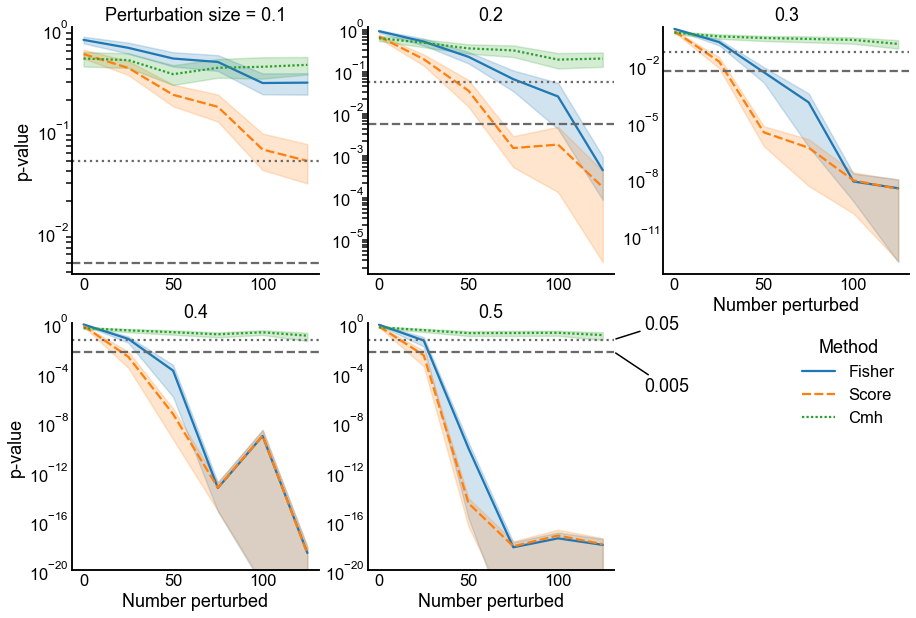
Fig. 8 p-values under the alternative for two different methods for combining p-values: Fisher’s method (performed on the uncorrected p-values) and Tippett’s method. The alternative is specified by changing the number of probabilities which are perturbed (x-axis in each panel) as well as the size of the perturbations which are done to each probability (panels show increasing perturbation size). Dotted and dashed lines indicate significance thresholds for \(\alpha = \{0.05, 0.005\}\), respectively. Note that in this simulation, even for large numbers of small perturbations (i.e. upper left panel), Tippett’s method has smaller p-values. Fisher’s method displays smaller p-values than Tippett’s only when there are many (>50) large perturbations, but by this point both methods yield extremely small p-values.#
Power under the alternative#
Show code cell source
alpha = 0.05
results["detected"] = 0
results.loc[results[(results["pvalue"] < alpha)].index, "detected"] = 1
Show code cell source
def shrink_axis(ax, scale=0.7):
    pos = ax.get_position()
    mid = (pos.ymax + pos.ymin) / 2
    height = pos.ymax - pos.ymin
    new_pos = Bbox(
        [
            [pos.xmin, mid - scale * 0.5 * height],
            [pos.xmax, mid + scale * 0.5 * height],
        ]
    )
    ax.set_position(new_pos)


def power_heatmap(
    data,
    ax=None,
    center=0,
    vmin=0,
    vmax=1,
    cmap="RdBu_r",
    cbar=False,
    labels=True,
    **kwargs,
):
    out = sns.heatmap(
        data.values[1:, 1:],
        ax=ax,
        yticklabels=perturb_size_range[1:],
        xticklabels=n_perturb_range[1:],
        square=True,
        center=center,
        vmin=vmin,
        vmax=vmax,
        cbar_kws=dict(shrink=0.7),
        cbar=cbar,
        cmap=cmap,
        **kwargs,
    )
    ax.invert_yaxis()
    if not labels:
        ax.set(xticklabels=[], yticklabels=[])
    return out
Show code cell source
fig, axs = plt.subplots(len(combine_methods), len(methods), figsize=(10, 10))
for i, combine_method in enumerate(combine_methods):
    for j, method in enumerate(methods):
        sub_results = results.query(
            "combine_method == @combine_method & method == @method"
        )
        sub_powers_square = sub_results.reset_index().pivot_table(
            index="perturb_size", columns="n_perturb", values="detected", aggfunc="mean"
        )
        power_heatmap(sub_powers_square, ax=axs[i, j])
        ax = axs[i, j]
        if i == 0:
            ax.set_title(method.capitalize())
        if j == 0:
            ax.set_ylabel(combine_method.capitalize())
/Users/bpedigo/JHU_code/bilateral/bilateral-connectome/.venv/lib/python3.9/site-packages/seaborn/matrix.py:305: UserWarning: Attempting to set identical left == right == 0 results in singular transformations; automatically expanding.
  ax.set(xlim=(0, self.data.shape[1]), ylim=(0, self.data.shape[0]))
/Users/bpedigo/JHU_code/bilateral/bilateral-connectome/.venv/lib/python3.9/site-packages/seaborn/matrix.py:305: UserWarning: Attempting to set identical bottom == top == 0 results in singular transformations; automatically expanding.
  ax.set(xlim=(0, self.data.shape[1]), ylim=(0, self.data.shape[0]))
Show code cell source
fig, axs = plt.subplots(
    len(combine_methods) * len(methods),
    len(combine_methods) * len(methods),
    figsize=(10, 10),
)

pal = sns.diverging_palette(145, 300, s=60, as_cmap=True)

for i, ((combine_method1, method1), sub_results1) in enumerate(
    results.groupby(["combine_method", "method"])
):
    sub_powers_square1 = sub_results1.reset_index().pivot_table(
        index="perturb_size", columns="n_perturb", values="detected", aggfunc="mean"
    )
    for j, ((combine_method2, method2), sub_results2) in enumerate(
        results.groupby(["combine_method", "method"])
    ):
        ax = axs[i, j]
        if i > j:
            sub_powers_square2 = sub_results2.reset_index().pivot_table(
                index="perturb_size",
                columns="n_perturb",
                values="detected",
                aggfunc=np.nanmean,
            )

            ratios_square = sub_powers_square1 / sub_powers_square2
            ratios_square.fillna(1, inplace=True)
            ratios_square[ratios_square == np.inf] = 1

            if np.nanmean(ratios_square.values) > 1:
                print(
                    f"{method1.capitalize()}, {combine_method1.capitalize()} > {method2.capitalize()}, {combine_method2.capitalize()}"
                )

            im = power_heatmap(
                np.log10(ratios_square),
                ax=ax,
                vmin=-2,
                vmax=2,
                center=0,
                cmap=pal,
                labels=False,
            )
        if i == j:
            null_results = sub_results1.query("perturb_size == 0.0 & n_perturb == 0")
            subuniformity_plot(
                null_results["pvalue"], ax=ax, legend=False, write_pvalue=False
            )
            ax.set(ylabel="", xlabel="", yticks=[])
        if i == 0:
            ax.set_title(f"{method2.capitalize()}, {combine_method2.capitalize()}")
        if j == 0:
            ax.set_ylabel(f"{method1.capitalize()}, {combine_method1.capitalize()}")
        if i < j:
            ax.axis("off")
        # else:
        #     ax.axis("off")

gluefig("power_validity_grid", fig)
Fisher, Fisher > Cmh, Cmh
/Users/bpedigo/JHU_code/bilateral/bilateral-connectome/.venv/lib/python3.9/site-packages/pandas/core/internals/blocks.py:352: RuntimeWarning: divide by zero encountered in log10
  result = func(self.values, **kwargs)
Score, Fisher > Cmh, Cmh
Score, Fisher > Fisher, Fisher
/Users/bpedigo/JHU_code/bilateral/bilateral-connectome/.venv/lib/python3.9/site-packages/pandas/core/internals/blocks.py:352: RuntimeWarning: divide by zero encountered in log10
  result = func(self.values, **kwargs)
Fisher, Tippett > Cmh, Cmh
Fisher, Tippett > Fisher, Fisher
/Users/bpedigo/JHU_code/bilateral/bilateral-connectome/.venv/lib/python3.9/site-packages/pandas/core/internals/blocks.py:352: RuntimeWarning: divide by zero encountered in log10
  result = func(self.values, **kwargs)
Fisher, Tippett > Score, Fisher
Score, Tippett > Cmh, Cmh
/Users/bpedigo/JHU_code/bilateral/bilateral-connectome/.venv/lib/python3.9/site-packages/pandas/core/internals/blocks.py:352: RuntimeWarning: divide by zero encountered in log10
  result = func(self.values, **kwargs)
Score, Tippett > Fisher, Fisher
Score, Tippett > Score, Fisher
Score, Tippett > Fisher, Tippett
Show code cell source
# fisher_results = results[results["method"] == "fisher"]
# min_results = results[results["method"] == "tippett"]
fisher_results = results.query("method == 'score' & combine_method == 'fisher'")
tippett_results = results.query("method == 'score' & combine_method == 'tippett'")

fisher_means = fisher_results.groupby(["perturb_size", "n_perturb"]).mean(
    numeric_only=True
)
min_means = tippett_results.groupby(["perturb_size", "n_perturb"]).mean(
    numeric_only=True
)

fisher_power_square = fisher_means.reset_index().pivot(
    index="perturb_size", columns="n_perturb", values="detected"
)
min_power_square = min_means.reset_index().pivot(
    index="perturb_size", columns="n_perturb", values="detected"
)

mean_diffs = fisher_means["detected"] / min_means["detected"]

mean_diffs = mean_diffs.to_frame().reset_index()

ratios_square = mean_diffs.pivot(
    index="perturb_size", columns="n_perturb", values="detected"
)

v = np.max(np.abs(mean_diffs.values))
Show code cell source
set_theme(font_scale=1.5)
# set up plot
pad = 0.5
width_ratios = [1, pad * 1.2, 10, pad, 10, 1.3 * pad, 10, 1]
fig, axs = plt.subplots(
    1,
    len(width_ratios),
    figsize=(30, 10),
    gridspec_kw=dict(
        width_ratios=width_ratios,
    ),
)
fisher_col = 2
min_col = 4
ratio_col = 6


ax = axs[fisher_col]
im = power_heatmap(fisher_power_square, ax=ax)
ax.set_title("Fisher's method", fontsize="large")

ax = axs[0]
shrink_axis(ax, scale=0.5)
_ = fig.colorbar(
    im.get_children()[0],
    cax=ax,
    fraction=1,
    shrink=1,
    ticklocation="left",
)
ax.set_title("Power\n" + r"($\alpha=0.05$)", pad=25)

ax = axs[min_col]
power_heatmap(min_power_square, ax=ax)
ax.set_title("Tippett's method", fontsize="large")
ax.set(yticks=[])

pal = sns.diverging_palette(145, 300, s=60, as_cmap=True)

ax = axs[ratio_col]
im = power_heatmap(np.log10(ratios_square), ax=ax, vmin=-2, vmax=2, center=0, cmap=pal)
ax.set(yticks=[])

ax = axs[-1]
shrink_axis(ax, scale=0.5)
_ = fig.colorbar(
    im.get_children()[0],
    cax=ax,
    fraction=1,
    shrink=1,
    ticklocation="right",
)
ax.text(2, 1, "Fisher more\nsensitive", transform=ax.transAxes, va="top")
ax.text(2, 0.5, "Equal power", transform=ax.transAxes, va="center")
ax.text(2, 0, "Tippett's more\nsensitive", transform=ax.transAxes, va="bottom")
ax.set_title("Log10\npower\nratio", pad=20)

# remove dummy axes
for i in range(len(width_ratios)):
    if not axs[i].has_data():
        axs[i].set_visible(False)

xlabel = r"# perturbed blocks $\rightarrow$"
ylabel = r"Perturbation size $\rightarrow$"
axs[fisher_col].set(
    xlabel=xlabel,
    ylabel=ylabel,
)
axs[min_col].set(xlabel=xlabel, ylabel="")
axs[ratio_col].set(xlabel=xlabel, ylabel="")

fig.text(0.09, 0.86, "A)", fontweight="bold", fontsize=50)
fig.text(0.64, 0.86, "B)", fontweight="bold", fontsize=50)
gluefig("relative_power", fig)
/Users/bpedigo/JHU_code/bilateral/bilateral-connectome/.venv/lib/python3.9/site-packages/pandas/core/internals/blocks.py:352: RuntimeWarning: divide by zero encountered in log10
  result = func(self.values, **kwargs)
Show code cell source
set_theme(font_scale=1.25)


min_null_results = tippett_results[
    (tippett_results["n_perturb"] == 0) | (tippett_results["perturb_size"] == 0)
]

fig, ax = plt.subplots(1, 1, figsize=(8, 8))
subuniformity_plot(min_null_results["pvalue"], ax=ax, write_pvalue=False)
ax.set_xlabel("p-value")
ax.set(title="p-values under $H_0$")
gluefig("tippett_null_cdf", fig)
Show code cell source
fig, ax = plt.subplots(1, 1, figsize=(8, 8))
out = power_heatmap(min_power_square, ax=ax, cbar=True)
xlabel = r"# perturbed blocks $(t)$ $\rightarrow$"
ylabel = r"Perturbation size $(\delta)$ $\rightarrow$"
ax.set(xlabel=xlabel, ylabel=ylabel, title="Power under $H_A $" + r"($\alpha=0.05$)")
gluefig("tippett_power_matrix", fig)
Show code cell source
fontsize = 12

null = SmartSVG(FIG_PATH / "tippett_null_cdf.svg")
null.set_width(200)
null.move(10, 10)
null_panel = Panel(null, Text("A)", 5, 10, size=fontsize, weight="bold"))

power = SmartSVG(FIG_PATH / "tippett_power_matrix.svg")
power.set_width(200)
power.move(20, 20)
power_panel = Panel(power, Text("B)", 5, 10, size=fontsize, weight="bold"))
power_panel.move(null.width * 0.9, 0)

fig = Figure(null.width * 2 * 0.9, null.width * 0.9, null_panel, power_panel)
fig.save(FIG_PATH / "tippett_sim_composite.svg")

svg_to_pdf(
    FIG_PATH / "tippett_sim_composite.svg", FIG_PATH / "tippett_sim_composite.pdf"
)

fig

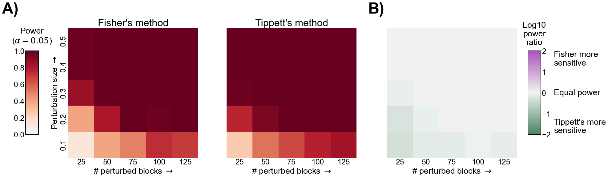
Fig. 9 Comparison of power for Fisher’s and Tippett’s method. A) The power under the alternative described in the text for both Fisher’s method and Tippett’s method. In both heatmaps, the x-axis represents an increasing number of blocks which are perturbed, and the y-axis represents an increasing magnitude for each perturbation. B) The log of the ratio of powers (Fisher’s / Tippett’s) for each alternative. Note that positive (purple) values would represent that Fisher’s is more powerful, and negative (green) represent that Tippett’s method is more powerful. Notice that Tippett’s method appears to have more power for subtler (fewer or smaller perturbations) alternatives, and nearly equal power for more obvious alternatives.#