Density test

Here, we compare the two unmatched networks by treating each as an Erdos-Renyi network and simply compare their estimated densities.

The Erdos-Renyi (ER) model

The Erdos-Renyi (ER) model is one of the simplest network models. This model treats the probability of each potential edge in the network occuring to be the same. In other words, all edges between any two nodes are equally likely.

Math

Let \(n\) be the number of nodes. We say that for all \((i, j), i \neq j\), with \(i\) and \(j\) both running from \(1 ... n\), the probability of the edge \((i, j)\) occuring is:

\[ P[A_{ij} = 1] = p_{ij} = p \]

Where \(p\) is the the global connection probability.

Each element of the adjacency matrix \(A\) is then sampled independently according to a Bernoulli distribution:

\[ A_{ij} \sim Bernoulli(p) \]

For a network modeled as described above, we say it is distributed

\[ A \sim ER(n, p) \]

Thus, for this model, the only parameter of interest is the global connection probability, \(p\). This is sometimes also referred to as the network density.

Testing under the ER model

In order to compare two networks \(A^{(L)}\) and \(A^{(R)}\) under this model, we simply need to compute these network densities (\(p^{(L)}\) and \(p^{(R)}\)), and then run a statistical test to see if these densities are significantly different.

Math

Under this model, the total number of edges \(m\) comes from a \(Binomial(n(n-1), p)\) distribution, where \(n\) is the number of nodes. This is because the number of edges is the sum of independent Bernoulli trials with the same probability. If \(m^{(L)}\) is the number of edges on the left hemisphere, and \(m^{(R)}\) is the number of edges on the right, then we have:

\[m^{(L)} \sim Binomial(n^{(L)}(n^{(L)} - 1), p^{(L)})\]

and independently,

\[m^{(R)} \sim Binomial(n^{(R)}(n^{(R)} - 1), p^{(R)})\]

To compare the two networks, we are just interested in a comparison of \(p^{(L)}\) vs. \(p^{(R)}\). Formally, we are testing:

\[H_0: p^{(L)} = p^{(R)}, \quad H_a: p^{(L)} \neq p^{(R)}\]

Fortunately, the problem of testing for equal proportions is well studied. In our case, we will use Fisher’s Exact test to run this test for the null and alternative hypotheses above.

Show code cell source Hide code cell source

import datetime
import time

import matplotlib.pyplot as plt
import numpy as np
import pandas as pd
import seaborn as sns
from pkg.data import load_network_palette, load_unmatched
from pkg.io import FIG_PATH, get_environment_variables
from pkg.io import glue as default_glue
from pkg.io import savefig
from pkg.plot import (
    SmartSVG,
    draw_hypothesis_box,
    merge_axes,
    networkplot_simple,
    plot_density,
    rainbowarrow,
    set_theme,
    soft_axis_off,
    svg_to_pdf,
)
from pkg.stats import erdos_renyi_test
from pkg.utils import sample_toy_networks
from svgutils.compose import Figure, Panel, Text

from graspologic.simulations import er_np

_, _, DISPLAY_FIGS = get_environment_variables()

FILENAME = "er_unmatched_test"


def gluefig(name, fig, **kwargs):
    savefig(name, foldername=FILENAME, **kwargs)

    glue(name, fig, figure=True)

    if not DISPLAY_FIGS:
        plt.close()


def glue(name, var, **kwargs):
    default_glue(name, var, FILENAME, **kwargs)


t0 = time.time()
set_theme(font_scale=1.25)

network_palette, NETWORK_KEY = load_network_palette()

left_adj, left_nodes = load_unmatched("left")
right_adj, right_nodes = load_unmatched("right")

Environment variables:
   RESAVE_DATA: true
   RERUN_SIMS: true
   DISPLAY_FIGS: False

Diagram of the ER model

Show code cell source Hide code cell source

np.random.seed(8888)
ps = [0.2, 0.4, 0.6]
n_steps = len(ps)
fig, axs = plt.subplots(
    2,
    n_steps,
    figsize=(6, 3),
    gridspec_kw=dict(height_ratios=[2, 0.5]),
    constrained_layout=True,
)
n = 18
for i, p in enumerate(ps):
    A = er_np(n, p)
    if i == 0:
        node_data = pd.DataFrame(index=np.arange(n))

    ax = axs[0, i]
    networkplot_simple(A, node_data, ax=ax, compute_layout=i == 0)

    label_text = f"{p}"
    if i == 0:
        label_text = r"$p = $" + label_text
    ax.set_title(label_text, pad=10)

fig.set_facecolor("w")


ax = merge_axes(fig, axs, rows=1)

soft_axis_off(ax)


rainbowarrow(ax, (0.15, 0.5), (0.85, 0.5), cmap="Blues", n=100, lw=12)
ax.set_xlim((0, 1))
ax.set_ylim((0, 1))
ax.set_xticks([])
ax.set_yticks([])
ax.set_xlabel("Increasing density")

gluefig("er_explain", fig)

Diagram of the density test

Show code cell source Hide code cell source

A1, A2, node_data = sample_toy_networks()
node_data["labels"] = np.ones(len(node_data), dtype=int)
palette = {1: sns.color_palette("Set2")[2]}
fig, axs = plt.subplots(2, 2, figsize=(6, 6), gridspec_kw=dict(wspace=0.7))

ax = axs[0, 0]
networkplot_simple(A1, node_data, ax=ax)

ax.set_title("Compute global\nconnection density")
ax.set_ylabel(
    "Left",
    color=network_palette["Left"],
    size="large",
    rotation=0,
    ha="right",
    labelpad=10,
)


ax = axs[1, 0]
networkplot_simple(A2, node_data, ax=ax)

ax.set_ylabel(
    "Right",
    color=network_palette["Right"],
    size="large",
    rotation=0,
    ha="right",
    labelpad=10,
)

stat, pvalue, misc = erdos_renyi_test(A1, A2)


ax = axs[0, 1]
ax.text(
    0.4,
    0.2,
    r"$p = \frac{\# \ edges}{\# \ potential \ edges}$",
    ha="center",
    va="center",
)
ax.axis("off")


ax.set_title("Compare ER\nmodels")
ax.set(xlim=(-0.5, 2), ylim=(0, 1))


ax = axs[1, 1]
ax.axis("off")

x = 0
y = 0.55


draw_hypothesis_box("er", -0.2, 0.8, ax=ax, fontsize="medium", yskip=0.2)


gluefig("er_methods", fig)

Show code cell source Hide code cell source

stat, pvalue, misc = erdos_renyi_test(left_adj, right_adj)
glue("pvalue", pvalue, form="pvalue")

Show code cell source Hide code cell source

n_possible_left = misc["possible1"]
n_possible_right = misc["possible2"]
glue("n_possible_left", n_possible_left, form="long")
glue("n_possible_right", n_possible_right, form="long")

density_left = misc["probability1"]
density_right = misc["probability2"]
glue("density_left", density_left, form="0.2g")
glue("density_right", density_right, form="0.2g")

density_ratio = density_left / density_right
glue("density_ratio", density_ratio, form="0.2f")

n_edges_left = misc["observed1"]
n_edges_right = misc["observed2"]

Show code cell source Hide code cell source

coverage = 0.95
glue("coverage", coverage, form="2.0f%")
plot_density(misc, palette=network_palette, coverage=coverage)

gluefig("er_density", fig)

Reject bilateral symmetry under the ER model

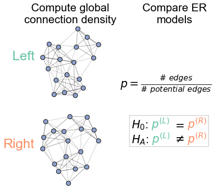
Fig. 3 Comparison of estimated densities for the left and right hemisphere networks. The estimated density (probability of any edge across the entire network), \(\hat{p}\), for the left hemisphere is ~0.016, while for the right it is ~0.017. Black lines denote % confidence intervals for this estimated parameter \(\hat{p}\). The p-value for testing the null hypothesis that these densities are the same is 4.87e-24 (two sided Fisher’s exact test).

Figure 3 shows the comparison of the network densities between the left and right hemisphere induced subgraphs. We see that the density on the left is ~0.016, and on the right it is ~0.017. To determine whether this is a difference likely to be observed by chance under the ER model, we ran a two-sided Fisher’s exact test, which tests whether the success probabilities between two independent binomials are significantly different. This test yields a p-value of 4.87e-24, suggesting that we have strong evidence to reject this version of our hypotheis of bilateral symmetry. We note that while the difference between estimated densities is not massive, this low p-value results from the large sample size for this comparison. We note that there are 2,266,530 and 2,266,530 potential edges on the left and right, respectively, making the sample size for this comparison quite large.

To our knowledge, when neuroscientists have considered the question of bilateral symmetry, they have not meant such a simple comparison of proportions. In many ways, the ER model is too simple to be an interesting description of connectome structure. However, we note that even the simplest network model yields a significant difference between brain hemispheres for this organism. It is unclear whether this difference in densities is biological (e.g. a result of slightly differing rates of development for this individual), an artifact of how the data was collected (e.g. technological limitations causing slightly lower reconstruction rates on the left hemisphere), or something else entirely. Still, the ER test results also provide important considerations for other tests. Almost any network statistic (e.g. clustering coefficient, number of triangles, etc), as well as many of the model-based parameters we will consider in this paper, are strongly related to the network density. Thus, if the densities are different, it is likely that tests based on any of these other test statistics will also reject the null hypothesis. Thus, we will need ways of telling whether an observed difference for these other tests could be explained by this difference in density alone.

Show code cell source Hide code cell source

FIG_PATH = FIG_PATH / FILENAME

fontsize = 9

methods = SmartSVG(FIG_PATH / "er_methods.svg")
methods.set_width(200)
methods.move(10, 20)
methods_panel = Panel(
    methods, Text("A) Density test methods", 5, 10, size=fontsize, weight="bold")
)

density = SmartSVG(FIG_PATH / "er_density.svg")
density.set_height(methods.height)
density.move(10, 15)
density_panel = Panel(
    density, Text("B) Density comparison", 5, 10, size=fontsize, weight="bold")
)
density_panel.move(methods.width * 0.9, 0)

fig = Figure(
    (methods.width + density.width) * 0.9,
    (methods.height) * 0.9,
    methods_panel,
    density_panel,
)
fig.save(FIG_PATH / "composite.svg")

svg_to_pdf(FIG_PATH / "composite.svg", FIG_PATH / "composite.pdf")

fig

End

Show code cell source Hide code cell source

elapsed = time.time() - t0
delta = datetime.timedelta(seconds=elapsed)
print(f"Script took {delta}")
print(f"Completed at {datetime.datetime.now()}")

Script took 0:00:05.677516
Completed at 2023-03-10 13:26:05.593312