Calculating CMI

import matplotlib.pyplot as plt
import numpy as np
import pandas as pd
import seaborn as sns
from scipy.stats import entropy

from sktree.datasets import make_trunk_classification
from sktree.ensemble import HonestForestClassifier
from sktree.stats import build_oob_forest
from sktree.tree import MultiViewDecisionTreeClassifier

sns.set(color_codes=True, style="white", context="talk", font_scale=1.5)
PALETTE = sns.color_palette("Set1")
sns.set_palette(PALETTE[1:5] + PALETTE[6:], n_colors=9)
sns.set_style("white", {"axes.edgecolor": "#dddddd"})

CMI

Conditional mutual information (CMI) measures the dependence of Y on X conditioned on Z. It can be calculated by the difference between the joint MI (I([X, Z]; Y)) and the MI on Z (I(Y; Z)):

\[I(X; Y | Z) = I([X, Z]; Y) - I(Y; Z)\]

With a multiview binary class simulation as an example, this tutorial will show how to use treeple to calculate the statistic with multiview data.

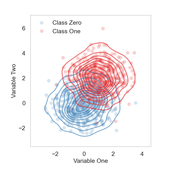
Create a simulation with two gaussians

# create a binary class simulation with two gaussians
# 500 samples for each class, class zero is standard
# gaussian, and class one has a mean at one for Z
Z, y = make_trunk_classification(
    n_samples=1000,
    n_dim=1,
    mu_0=0,
    mu_1=1,
    n_informative=1,
    seed=1,
)

# class one has a mean at two for X
X, y = make_trunk_classification(
    n_samples=1000,
    n_dim=1,
    mu_0=0,
    mu_1=2,
    n_informative=1,
    seed=2,
)

Z_X = np.hstack((Z, X))


Z_X_y = np.hstack((Z_X, y.reshape(-1, 1)))
Z_X_y = pd.DataFrame(Z_X_y, columns=["Z", "X", "y"])
Z_X_y = Z_X_y.replace({"y": 0.0}, "Class Zero")
Z_X_y = Z_X_y.replace({"y": 1.0}, "Class One")

fig, ax = plt.subplots(figsize=(6, 6))
fig.tight_layout()
ax.tick_params(labelsize=15)
sns.scatterplot(data=Z_X_y, x="Z", y="X", hue="y", palette=PALETTE[:2][::-1], alpha=0.2)
sns.kdeplot(data=Z_X_y, x="Z", y="X", hue="y", palette=PALETTE[:2][::-1], alpha=0.6)
ax.set_ylabel("Variable Two", fontsize=15)
ax.set_xlabel("Variable One", fontsize=15)
plt.legend(frameon=False, fontsize=15)

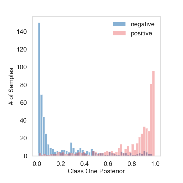
Fit the model with X and Z

# initialize the forest with 100 trees
est = HonestForestClassifier(
    n_estimators=100,
    max_samples=1.6,
    max_features=0.3,
    bootstrap=True,
    stratify=True,
    tree_estimator=MultiViewDecisionTreeClassifier(),
    random_state=1,
)

# fit the model and obtain the tree posteriors
_, observe_proba = build_oob_forest(est, Z_X, y)

# generate forest posteriors for the two classes
observe_proba = np.nanmean(observe_proba, axis=0)


fig, ax = plt.subplots(figsize=(6, 6))
fig.tight_layout()
ax.tick_params(labelsize=15)

# histogram plot the posterior probabilities for class one
ax.hist(observe_proba[:500][:, 1], bins=50, alpha=0.6, color=PALETTE[1], label="negative")
ax.hist(observe_proba[500:][:, 1], bins=50, alpha=0.3, color=PALETTE[0], label="positive")
ax.set_ylabel("# of Samples", fontsize=15)
ax.set_xlabel("Class One Posterior", fontsize=15)
plt.legend(frameon=False, fontsize=15)
plt.show()

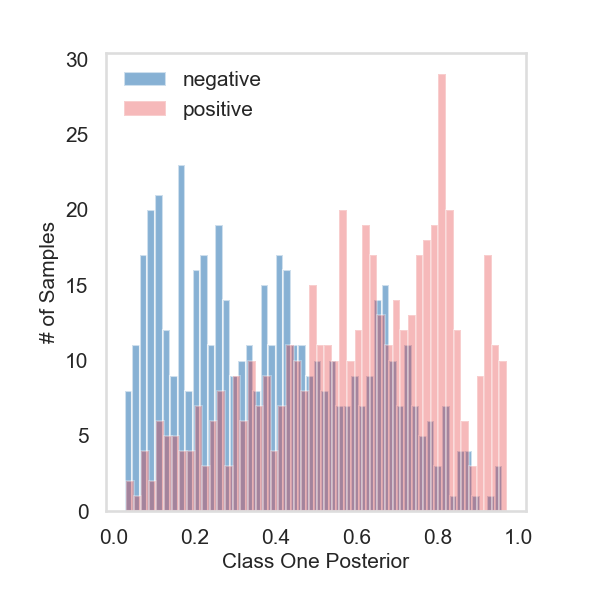
Fit the model with Z only

# initialize the forest with 100 trees
est = HonestForestClassifier(
    n_estimators=100,
    max_samples=1.6,
    max_features=0.3,
    bootstrap=True,
    stratify=True,
    random_state=1,
)

# fit the model and obtain the tree posteriors
_, single_proba = build_oob_forest(est, Z, y)

# generate forest posteriors for the two classes
single_proba = np.nanmean(single_proba, axis=0)


fig, ax = plt.subplots(figsize=(6, 6))
fig.tight_layout()
ax.tick_params(labelsize=15)

# histogram plot the posterior probabilities for class one
ax.hist(single_proba[:500][:, 1], bins=50, alpha=0.6, color=PALETTE[1], label="negative")
ax.hist(single_proba[500:][:, 1], bins=50, alpha=0.3, color=PALETTE[0], label="positive")
ax.set_ylabel("# of Samples", fontsize=15)
ax.set_xlabel("Class One Posterior", fontsize=15)
plt.legend(frameon=False, fontsize=15)
plt.show()

Calculate the statistic

def Calculate_MI(y_true, y_pred_proba):
    # calculate the conditional entropy
    H_YX = np.mean(entropy(y_pred_proba, base=np.exp(1), axis=1))

    # empirical count of each class (n_classes)
    _, counts = np.unique(y_true, return_counts=True)
    # calculate the entropy of labels
    H_Y = entropy(counts, base=np.exp(1))
    return H_Y - H_YX


joint_mi = Calculate_MI(y, observe_proba)
mi = Calculate_MI(y, single_proba)

print("CMI =", round(joint_mi - mi, 2))

CMI = 0.23