Calculating Hellinger Distance

import matplotlib.pyplot as plt
import numpy as np
import seaborn as sns

from sktree.datasets import make_trunk_classification
from sktree.ensemble import HonestForestClassifier
from sktree.stats import build_oob_forest

sns.set(color_codes=True, style="white", context="talk", font_scale=1.5)
PALETTE = sns.color_palette("Set1")
sns.set_palette(PALETTE[1:5] + PALETTE[6:], n_colors=9)
sns.set_style("white", {"axes.edgecolor": "#dddddd"})

Hellinger Distance

Hellinger distance quantifies the similarity between the two posterior probability distributions (class zero and class one).

\[H(\eta(X), 1-\eta(X)) = \frac{1}{\sqrt{2}} \; \bigl\|\sqrt{\eta(X)} - \sqrt{1-\eta(X)} \bigr\|_2\]

With a binary class simulation as an example, this tutorial will show how to use treeple to calculate the statistic.

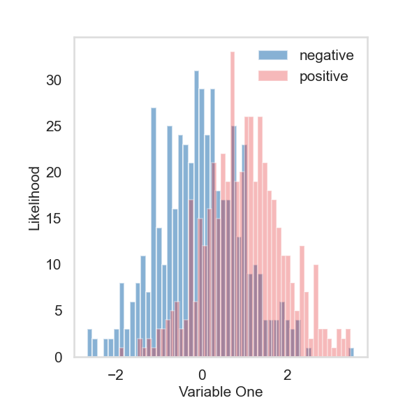
Create a simulation with two gaussians

# create a binary class simulation with two gaussians
# 500 samples for each class, class zero is standard
# gaussian, and class one has a mean at one
X, y = make_trunk_classification(
    n_samples=1000,
    n_dim=1,
    mu_0=0,
    mu_1=1,
    n_informative=1,
    seed=1,
)


fig, ax = plt.subplots(figsize=(6, 6))
fig.tight_layout()
ax.tick_params(labelsize=15)

# histogram plot the samples
ax.hist(X[:500], bins=50, alpha=0.6, color=PALETTE[1], label="negative")
ax.hist(X[500:], bins=50, alpha=0.3, color=PALETTE[0], label="positive")
ax.set_xlabel("Variable One", fontsize=15)
ax.set_ylabel("Likelihood", fontsize=15)
plt.legend(frameon=False, fontsize=15)
plt.show()

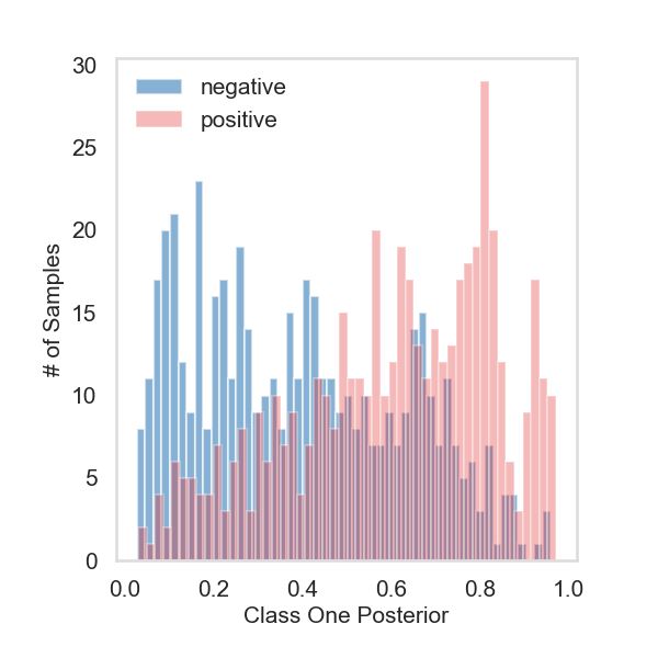
Fit the model

# initialize the forest with 100 trees
est = HonestForestClassifier(
    n_estimators=100,
    max_samples=1.6,
    max_features=0.3,
    bootstrap=True,
    stratify=True,
    random_state=1,
)

# fit the model and obtain the tree posteriors
_, observe_proba = build_oob_forest(est, X, y)

# generate forest posteriors for the two classes
observe_proba = np.nanmean(observe_proba, axis=0)


fig, ax = plt.subplots(figsize=(6, 6))
fig.tight_layout()
ax.tick_params(labelsize=15)

# histogram plot the posterior probabilities for class one
ax.hist(observe_proba[:500][:, 1], bins=50, alpha=0.6, color=PALETTE[1], label="negative")
ax.hist(observe_proba[500:][:, 1], bins=50, alpha=0.3, color=PALETTE[0], label="positive")
ax.set_ylabel("# of Samples", fontsize=15)
ax.set_xlabel("Class One Posterior", fontsize=15)
plt.legend(frameon=False, fontsize=15)
plt.show()

Calculate the statistic

def Calculate_hd(y_pred_proba) -> float:
    return np.sqrt(
        np.sum((np.sqrt(y_pred_proba[:, 1]) - np.sqrt(y_pred_proba[:, 0])) ** 2)
    ) / np.sqrt(2)


hd = Calculate_hd(observe_proba)
print("Hellinger distance =", round(hd, 2))

Hellinger distance = 8.81