Demonstrate Conditional Mutual Information for Genuine Hypothesis Testing (Co-MIGHT)

In this example, we demonstrate how to test the conditional mutual information (CMI) hypothesis test. To perform CMI testing, we have the hypothesis test:

• $H_0: I(X_2; Y | X_1) = 0$

• $H_1: I(X_2; Y | X_1) > 0$

Here, we simulate two feature-sets, which are both informative for the target. The data-generating process follows the graphical model:

$(X_1 rightarrow X_2 rightarrow Y; X_1 rightarrow Y)$

This means that $I(X_1; Y | X_2) > 0$ if we had a perfect estimate of CMI.

We will demonstrate how to perform the CMI test properly using a conditional permutation (compared to a standard permutation) of samples. We specifically explore the case where the alternative hypothesis is true and determine when the test is able to reject the null hypothesis correctly.

Note

This does not exactly implement conditional-independence testing yet, since we do not have a way to estimate the null distribution of $I(X_2; Y | X_1)$. However, we can still demonstrate the power of the test in the case where the alternative hypothesis is true.

import matplotlib.pyplot as plt
import numpy as np
from sklearn.datasets import make_spd_matrix

from sktree import HonestForestClassifier
from sktree.datasets import make_gaussian_mixture
from sktree.stats import FeatureImportanceForestClassifier
from sktree.tree import DecisionTreeClassifier, MultiViewDecisionTreeClassifier

seed = 12345
rng = np.random.default_rng(seed)

Simulate data

We simulate the two feature sets, and the target variable. We then combine them into a single dataset to perform hypothesis testing.

seed = 12345
rng = np.random.default_rng(seed)

n_samples = 200

n_features = 20
noise_dims = 80
class_probs = [0.6, 0.4]
n_features_2 = 1000 - noise_dims

fixed_center = rng.standard_normal(size=(n_features,))
centers = [fixed_center, fixed_center]

covariances = [
    make_spd_matrix(n_dim=n_features, random_state=seed),
    make_spd_matrix(n_dim=n_features, random_state=seed + 123),
]

Xs, y = make_gaussian_mixture(
    centers,
    covariances,
    n_samples=n_samples,
    noise=1.0,
    noise_dims=noise_dims,
    shuffle=True,
    class_probs=class_probs,
    random_state=seed,
    transform="linear",
)

second_X = Xs[0]
first_X = Xs[1]

print(first_X.shape, second_X.shape)
X = np.hstack((first_X, second_X, rng.standard_normal(size=(n_samples, n_features_2 - n_features))))
n_features_ends = [
    n_features + noise_dims,
    n_features_2 + n_features + noise_dims * 2,
]

print(X.shape, y.shape, n_features_ends)

(200, 100) (200, 100)
(200, 1100) (200,) [100, 1100]

Perform hypothesis testing

Here, we use FeatureImportanceForestClassifier to perform the hypothesis test. The test statistic is computed by comparing the metric (i.e. mutual information) estimated between two forests. One forest is trained on the original dataset, and one forest is trained on a permuted dataset, where the rows of the covariate_index columns are shuffled randomly.

The null distribution is then estimated in an efficient manner using the framework of [1]. The sample evaluations of each forest (i.e. the posteriors) are sampled randomly n_repeats times to generate a null distribution. The pvalue is then computed as the proportion of samples in the null distribution that are less than the observed test statistic.

n_estimators = 200
max_features = 0.3
test_size = 0.2
n_repeats = 1000
n_jobs = -1

est = FeatureImportanceForestClassifier(
    estimator=HonestForestClassifier(
        n_estimators=n_estimators,
        max_features=max_features,
        tree_estimator=MultiViewDecisionTreeClassifier(
            feature_set_ends=n_features_ends,
            apply_max_features_per_feature_set=True,
        ),
        random_state=seed,
        honest_fraction=0.5,
        n_jobs=n_jobs,
    ),
    random_state=seed,
    test_size=test_size,
    sample_dataset_per_tree=False,
)

mv_results = dict()

# we test for the first feature set, which is lower-dimensional
covariate_index = np.arange(n_features_ends[0], dtype=int)
stat, pvalue = est.test(X, y, covariate_index=covariate_index, metric="mi", n_repeats=n_repeats)

mv_results["low_dim_feature_stat"] = stat
mv_results["low_dim_feature_pvalue"] = pvalue
print("Analysis with multi-view decision tree.")
print(f"Estimated MI difference: {stat} with Pvalue: {pvalue}")

# we test for the second feature set, which is higher-dimensional
covariate_index = np.arange(n_features_ends[0], n_features_ends[1], dtype=int)
stat, pvalue = est.test(
    X,
    y,
    covariate_index=covariate_index,
    metric="mi",
    n_repeats=n_repeats,
)
mv_results["high_dim_feature_stat"] = stat
mv_results["high_dim_feature_pvalue"] = pvalue
print(f"Estimated MI difference: {stat} with Pvalue: {pvalue}")

Analysis with multi-view decision tree.
Estimated MI difference: -0.009960233587969936 with Pvalue: 0.000999000999000999
Estimated MI difference: 0.0007188967304878613 with Pvalue: 0.6153846153846154

Let’s investigate what happens when we do not use a multi-view decision tree. All other parameters are kept the same.

est = FeatureImportanceForestClassifier(
    estimator=HonestForestClassifier(
        n_estimators=n_estimators,
        max_features=max_features,
        tree_estimator=DecisionTreeClassifier(),
        random_state=seed,
        honest_fraction=0.5,
        n_jobs=n_jobs,
    ),
    random_state=seed,
    test_size=test_size,
    sample_dataset_per_tree=False,
)

rf_results = dict()

# we test for the first feature set, which is lower-dimensional
covariate_index = np.arange(n_features_ends[0], dtype=int)
stat, pvalue = est.test(X, y, covariate_index=covariate_index, metric="mi", n_repeats=n_repeats)

rf_results["low_dim_feature_stat"] = stat
rf_results["low_dim_feature_pvalue"] = pvalue
print("\n\nAnalysing now with a regular decision-tree")
print(f"Estimated MI difference using regular decision-trees: {stat} with Pvalue: {pvalue}")

# we test for the second feature set, which is higher-dimensional
covariate_index = np.arange(n_features_ends[0], n_features_ends[1], dtype=int)
stat, pvalue = est.test(
    X,
    y,
    covariate_index=covariate_index,
    metric="mi",
    n_repeats=n_repeats,
)
rf_results["high_dim_feature_stat"] = stat
rf_results["high_dim_feature_pvalue"] = pvalue
print(f"Estimated MI difference using regular decision-trees: {stat} with Pvalue: {pvalue}")

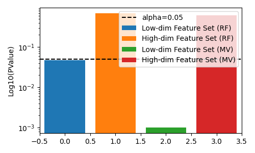
fig, ax = plt.subplots(figsize=(5, 3))

# plot pvalues
ax.bar(0, rf_results["low_dim_feature_pvalue"], label="Low-dim Feature Set (RF)")
ax.bar(1, rf_results["high_dim_feature_pvalue"], label="High-dim Feature Set (RF)")
ax.bar(2, mv_results["low_dim_feature_pvalue"], label="Low-dim Feature Set (MV)")
ax.bar(3, mv_results["high_dim_feature_pvalue"], label="High-dim Feature Set (MV)")
ax.axhline(0.05, color="k", linestyle="--", label="alpha=0.05")
ax.set(ylabel="Log10(PValue)", xlim=[-0.5, 3.5], yscale="log")
ax.legend()

fig.tight_layout()
plt.show()

Analysing now with a regular decision-tree
Estimated MI difference using regular decision-trees: -0.00441089991602206 with Pvalue: 0.04695304695304695
Estimated MI difference using regular decision-trees: 0.0011456756025775006 with Pvalue: 0.6863136863136863

Discussion

In this example, since both feature-sets are in informative for the target, the true answer should be reject the null hypothesis. We see that neither the regular decision tree, nor the multi-view decision tree is able to reject the null hypothesis correctly.

However, if we permute the lower-dimensional feature-set, the multi-view decision tree has a lower pvalue than the regular decision tree, which allows us to correctly reject the null hypothesis at lower $alpha$ levels.

References

[1]

Tim Coleman, Wei Peng, and Lucas Mentch. Scalable and efficient hypothesis testing with random forests. The Journal of Machine Learning Research, 23(1):7679–7713, 2022.