Replicate Fig 1
Replicate Fig 1#
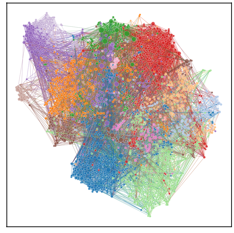
In this notebook we will be replicating figure 1 of the paper Whole-animal connectome and cell-type complement of the three-segmented Platynereis dumerilii larva, which is a network plot of the neurons in the larva’s connectome
import os
import logging
import pandas as pd
import numpy as np
import networkx as nx
from itertools import chain, combinations
from upsetplot import plot
from matplotlib import pyplot as plt
from networkx import from_numpy_array, number_of_nodes, number_of_edges, density
from graspologic.embed import AdjacencySpectralEmbed
from graspologic.layouts import layout_tsne, layout_umap
from graspologic.plot.plot import networkplot
from graspologic.utils import is_fully_connected, largest_connected_component, is_symmetric, symmetrize
from pkg.platy import load_connectome_adj, _get_folder
/Users/kareefullah/Library/Caches/pypoetry/virtualenvs/platy-data-EVeqgmAk-py3.9/lib/python3.9/site-packages/tqdm/auto.py:22: TqdmWarning: IProgress not found. Please update jupyter and ipywidgets. See https://ipywidgets.readthedocs.io/en/stable/user_install.html
  from .autonotebook import tqdm as notebook_tqdm
        skids side class segment   type  group
0     2015233    l     s    head  100.0    NaN
1     1548290    l   NaN       1    NaN    NaN
2     1318919    l     s    head   88.0   15.0
3     2015241    l     s    head  100.0    NaN
4     1646603    r   NaN       3    NaN    NaN
...       ...  ...   ...     ...    ...    ...
2696  1302513    l     s    head    NaN    NaN
2697  1630186    l   NaN       2    NaN    NaN
2698  1441779    r   NaN    head    NaN    NaN
2699  1671147    r     m       1  165.0    NaN
2700  1048573    l     i       3    NaN    NaN

[2701 rows x 6 columns]
      skids side class   segment   type  group
0   2007060   lr     i      head    NaN    NaN
1    139303   lr     s         1  102.0    NaN
2   2007344    l    im      head  166.0    NaN
3   1016172    l    im         1    NaN    NaN
4   1999932    r    sm         1   95.0    NaN
5   1320159   rc     i      head    NaN    NaN
6   1631592   lc   NaN  pygidium    NaN    NaN
7   1418928   lc     s      head  132.0    NaN
8   1320798   lc     s      head    NaN    NaN
9    370978    r    sm  pygidium   54.0    9.0
10    84457   rc   NaN      head    NaN    NaN
11  1462145    l    im         1    NaN    NaN
12   307194   rc     s      head  135.0    NaN
13  1462664   rc   NaN         2    NaN    NaN
14  1594313    r    sm  pygidium   93.0    9.0
15  1332516   rc     s      head   49.0    NaN
16  1366160   rc     i  pygidium    NaN    1.0
17    64258   lr     s         1   36.0    NaN
18  1276971    l    sm         2   80.0    NaN
19    81251   lc     s      head   43.0    NaN
20  1302189    r    im      head   11.0    NaN
21  1294206   lc     i      head    NaN    NaN
folder = _get_folder()
We import the adjacency matrix for the connection of connectome neurons and save its edgelist (note: we are working with a directed graph)
adj = load_connectome_adj()
g = nx.from_pandas_adjacency(adj, create_using=nx.DiGraph)
nx.write_edgelist(g, folder / "weighted_edgelist.csv")
To be able to make a network plot of the connectome neurons, we need to extract the largest connected component of the neurons, as there are a few neurons that have a degree of 0 (no incident edges), which we cannot plot
#numpy representation of original graph
adj_numpy_orig = adj.to_numpy()

#numpy largest connected component
adj_numpy_lcc, new_inds = largest_connected_component(adj_numpy_orig, return_inds=True)
#symmetrized version of numpy_lcc
adj_numpy_sym_lcc = symmetrize(adj_numpy_lcc)

#networkx representation of symmetrized lcc graph
adj_nx_sym_lcc = nx.from_numpy_array(adj_numpy_sym_lcc, create_using=nx.DiGraph)
print(adj_nx_sym_lcc)
DiGraph with 2723 nodes and 21691 edges
#use layout_tsne to get 2d representation of graph
X, node_pos = layout_tsne(adj_nx_sym_lcc, perplexity=100, n_iter=10000)
x_pos = []
y_pos = []
node_comms = []
for pos in node_pos:

    #save the assigned community of the node
    node_comms.append(pos[4])
    x_pos.append(pos[1])
    y_pos.append(pos[2])

node_comms = np.array(node_comms)
x_pos = np.array(x_pos)
y_pos = np.array(y_pos)
degrees = np.sum(adj_numpy_sym_lcc, axis=0)
/Users/kareefullah/Library/Caches/pypoetry/virtualenvs/platy-data-EVeqgmAk-py3.9/lib/python3.9/site-packages/sklearn/manifold/_t_sne.py:800: FutureWarning: The default initialization in TSNE will change from 'random' to 'pca' in 1.2.
  warnings.warn(
/Users/kareefullah/Library/Caches/pypoetry/virtualenvs/platy-data-EVeqgmAk-py3.9/lib/python3.9/site-packages/sklearn/manifold/_t_sne.py:810: FutureWarning: The default learning rate in TSNE will change from 200.0 to 'auto' in 1.2.
  warnings.warn(
WARNING:graspologic.layouts.auto:Directed graph converted to undirected graph for community detection
plot = networkplot(
    adjacency=adj_numpy_sym_lcc,
    x=x_pos,
    y=y_pos,
    node_hue=node_comms,
    palette="tab20",
    node_size=degrees,
    node_sizes=(20, 200),
    edge_hue="source",
    edge_alpha=0.5,
    edge_linewidth=0.5,
)
plt.savefig(folder / "tsne_connectome.png")
plt.show()
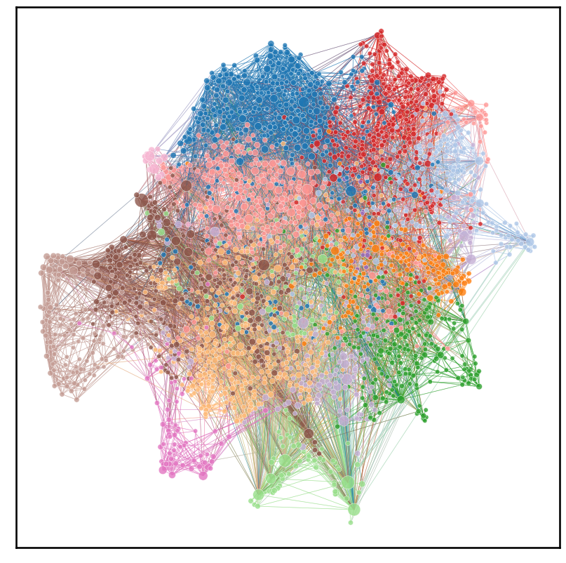
#use layout_umap to get 2d representation of graph
X, node_pos = layout_umap(adj_nx_sym_lcc)
x_pos = []
y_pos = []
node_comms = []
for pos in node_pos:
    node_comms.append(pos[4])
    x_pos.append(pos[1])
    y_pos.append(pos[2])

node_comms = np.array(node_comms)
x_pos = np.array(x_pos)
y_pos = np.array(y_pos)
degrees = np.sum(adj_numpy_sym_lcc, axis=0)
WARNING:graspologic.layouts.auto:Directed graph converted to undirected graph for community detection
plot = networkplot(
    adjacency=adj_numpy_sym_lcc,
    x=x_pos,
    y=y_pos,
    node_hue=node_comms,
    palette="tab20",
    node_size=degrees,
    node_sizes=(20, 200),
    edge_hue="source",
    edge_alpha=0.5,
    edge_linewidth=0.5,
)
plt.savefig(folder / "umap_connectome.png")
plt.show()
We are now interested in displaying the statistics from the graph we generated to that of the statistics given in table 1 of the paper, and we wish to make sure that our numbers are approximately the same
#given the adjacency matrix and a partition of the nodes return the modularity score
def modularity_from_adjacency(sym_adj, partition, resolution=1):
    if isinstance(partition, dict):
        partition_labels = np.vectorize(partition.__getitem__)(
            np.arange(sym_adj.shape[0])
        )
    else:
        partition_labels = partition
    partition_labels = np.array(partition_labels)
    in_comm_mask = partition_labels[:, None] == partition_labels[None, :]
    degrees = np.squeeze(np.asarray(sym_adj.sum(axis=0)))
    degree_prod_mat = np.outer(degrees, degrees) / sym_adj.sum()
    mod_mat = sym_adj - resolution * degree_prod_mat
    return mod_mat[in_comm_mask].sum() / sym_adj.sum()
#get original networkx graph (not lcc)
adj_nx_orig = nx.from_numpy_array(adj_numpy_orig, create_using=nx.DiGraph)

#stats on original graph
n_nodes_orig = adj_nx_orig.number_of_nodes()
n_edges_orig = adj_nx_orig.number_of_edges()
dens_orig = density(adj_nx_orig)

#cannot calc modularity because there are isolate nodes
mod_score_orig = "N/A"

avg_degree_orig = np.average(np.count_nonzero(adj_numpy_orig, axis=0))
avg_degree_orig
4.234237536656892
#get non-symmetrized lcc networkx graph
adj_nx_lcc = nx.from_numpy_array(adj_numpy_lcc, create_using=nx.DiGraph)

#stats on lcc adj
n_nodes_lcc = adj_nx_lcc.number_of_nodes()
n_edges_lcc = adj_nx_lcc.number_of_edges()
dens_lcc = density(adj_nx_lcc)

#make symmetric when calc mod
sym_adj_lcc = symmetrize(adj_numpy_lcc)
mod_score_lcc = modularity_from_adjacency(sym_adj_lcc, node_comms)

avg_degree_lcc = np.average(np.count_nonzero(adj_numpy_lcc, axis=0))
#paper stats
n_nodes_paper = 2728
n_edges_paper = 11437
dens_paper = 0.0015
mod_score_paper = 0.62
avg_degree_paper = 4.1
stats = {"Number of nodes": [n_nodes_orig, n_nodes_lcc, n_nodes_paper], "Number of edges": [n_edges_orig, n_edges_lcc, n_edges_paper], "Graph density": [dens_orig, dens_lcc, dens_paper], "Modularity": [mod_score_orig, mod_score_lcc, mod_score_paper], "Avg. degree": [avg_degree_orig, avg_degree_lcc, avg_degree_paper]}
stats_df = pd.DataFrame.from_dict(stats, orient="index", columns=["Orig adj", "LCC adj", "Paper"])
stats_df.to_csv(folder / "fig_1_stats.csv")
stats_df
| Orig adj | LCC adj | Paper | |
|---|---|---|---|
| Number of nodes | 2728 | 2723.000000 | 2728.0000 |
| Number of edges | 11551 | 11551.000000 | 11437.0000 |
| Graph density | 0.001553 | 0.001558 | 0.0015 |
| Modularity | N/A | 0.647185 | 0.6200 |
| Avg. degree | 4.234238 | 4.242012 | 4.1000 |
Looks like the values of our statistics very closely match those of the paper!