Matched Networks
Contents
### import modules
import numpy as np
import seaborn as sns
import matplotlib.pyplot as plt
import random
import pandas as pd
from sklearn.metrics import adjusted_rand_score, accuracy_score
from graspologic.utils import remap_labels
from utils import calculate_dissim, cluster_dissim, construct_df, plot_clustering, laplacian_dissim
from myst_nb import glue
Matched Networks
Here we will use some well-known clustering algorithms (Agglomerative clustering, GMM, KMeans) to cluster networks on the dissimilarity matrices that we generated.
To assess the performance of each clustering method, we calculate the adjusted rand index (ARI) and compare them. The rand index (RI) is a measure of how similar the predicted clusters are to the true, and the ARI is the raw RI value adjusted for chance. Thus, the ARI value is close to 0 for random labeling and close to 1 for accurate predictions.
Note that by default, we only show the result for Agglomerative clustering on the dissimilarity matrix constructed by the Edge weight kernel (\(L^2\)-norm), but all results can be expanded for viewing.
Load Data
# HIDE CELL
from graspologic.datasets import load_mice
random.seed(3)

# Load the full mouse dataset
mice = load_mice()

# Stack all adjacency matrices in a 3D numpy array
graphs = np.array(mice.graphs)
print(graphs.shape)

# construct labels
labels = mice.labels

mapper = {'B6': 0, 'BTBR': 1, 'CAST': 2, 'DBA2': 3}
y = np.array([mapper[l] for l in list(labels)])
(32, 332, 332)
Agglomerative Clustering
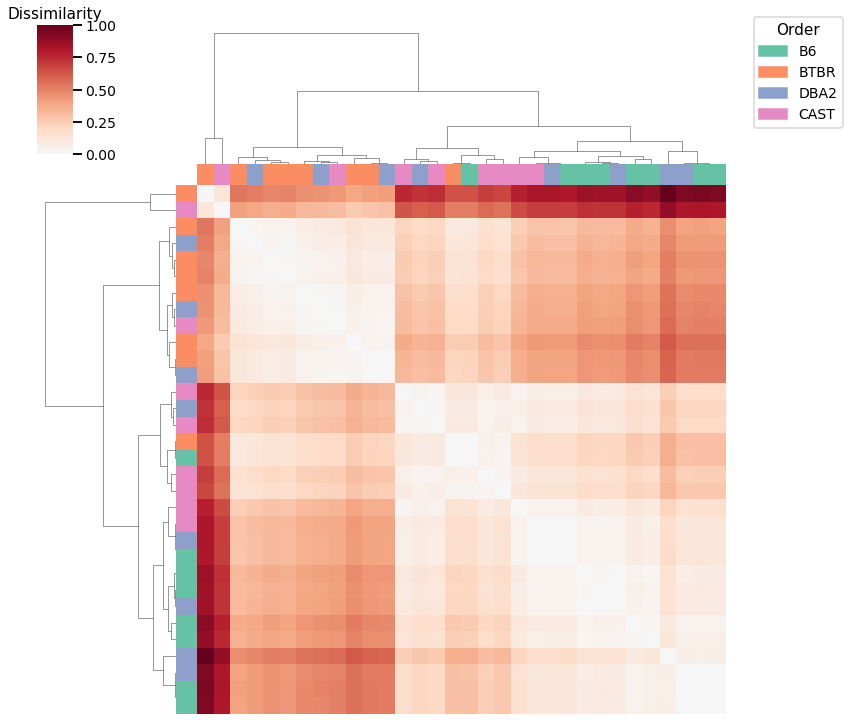
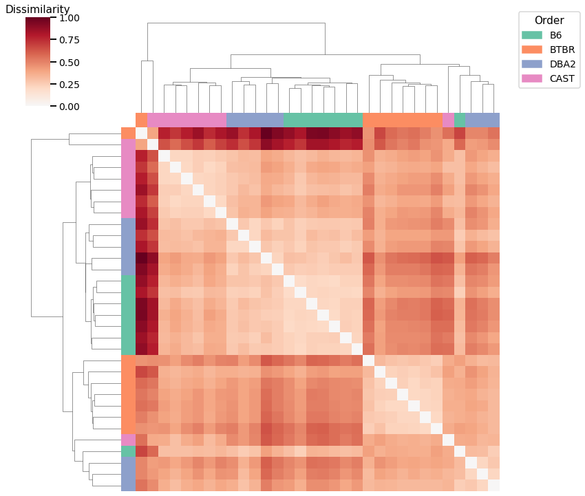
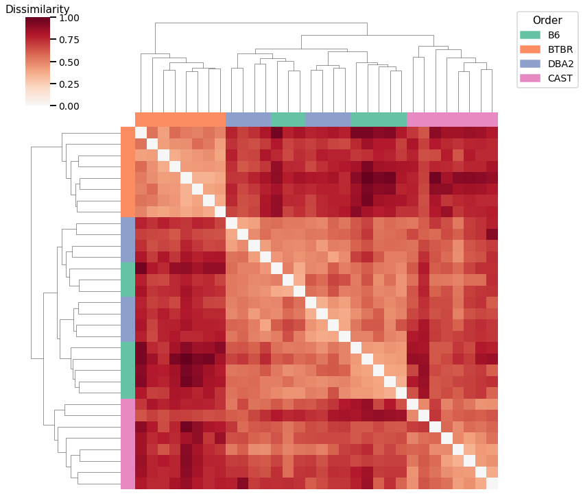
Here we use agglomerative clustering to cluster the graphs directly on the dissimilarity matrix, and the calculated linkage matrix and clusters are visualized with a heatmap below.
For each kernel, we report the accuracy score, the number of correct predictions divided by the total number of samples, and the adjusted rand index.
Density
# HIDE CELL
# calculate dissimilarity matrix
scaled_density_dissim = calculate_dissim(graphs, method="density", norm=None, normalize=True)

# cluster dissimilarity matrix
density_linkage_matrix, density_pred = cluster_dissim(scaled_density_dissim, y, method="agg", n_components=4)

# calculate accuracy and ARI
density_pred = remap_labels(y, density_pred)
density_agg_score = accuracy_score(y, density_pred)
density_agg_ari = adjusted_rand_score(y, density_pred)

print(f"Accuracy: {density_agg_score}")
print(f"ARI: {density_agg_ari}")

# plot clustered dissimilarity matrix
plot_clustering(labels, 'agg', scaled_density_dissim, density_linkage_matrix)
Accuracy: 0.53125
ARI: 0.20111167256189996
<seaborn.matrix.ClusterGrid at 0x7fdda07719a0>
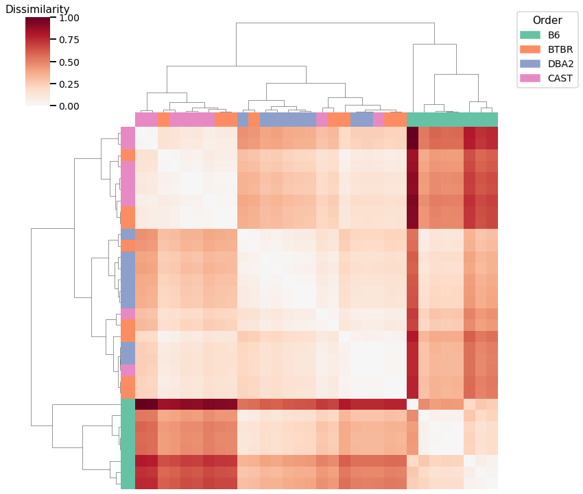
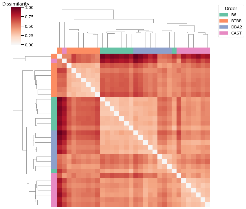
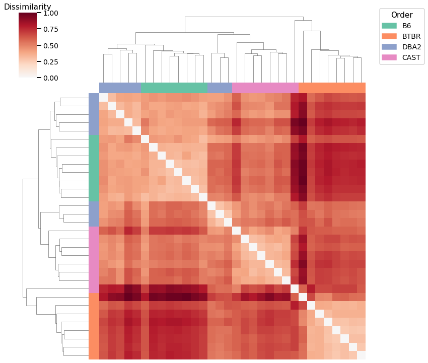
Average Edge Weight
# HIDE CELL
# calculate dissimilarity matrix
scaled_avgedgeweight_dissim = calculate_dissim(graphs, method="avgedgeweight", norm=None, normalize=True)

# cluster dissimilarity matrix
avgedgeweight_linkage_matrix, avgedgeweight_pred = cluster_dissim(scaled_avgedgeweight_dissim, y, method="agg", n_components=4)

# calculate accuracy and ARI
avgedgeweight_pred = remap_labels(y, avgedgeweight_pred)
avgedgeweight_agg_score = accuracy_score(y, avgedgeweight_pred)
avgedgeweight_agg_ari = adjusted_rand_score(y, avgedgeweight_pred)

print(f"Accuracy: {avgedgeweight_agg_score}")
print(f"ARI: {avgedgeweight_agg_ari}")

# plot clustered dissimilarity matrix
fig = plot_clustering(labels, 'agg', scaled_avgedgeweight_dissim, avgedgeweight_linkage_matrix)
Accuracy: 0.65625
ARI: 0.4124638612271121
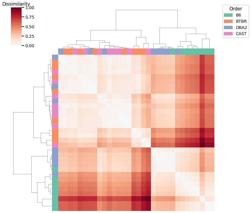
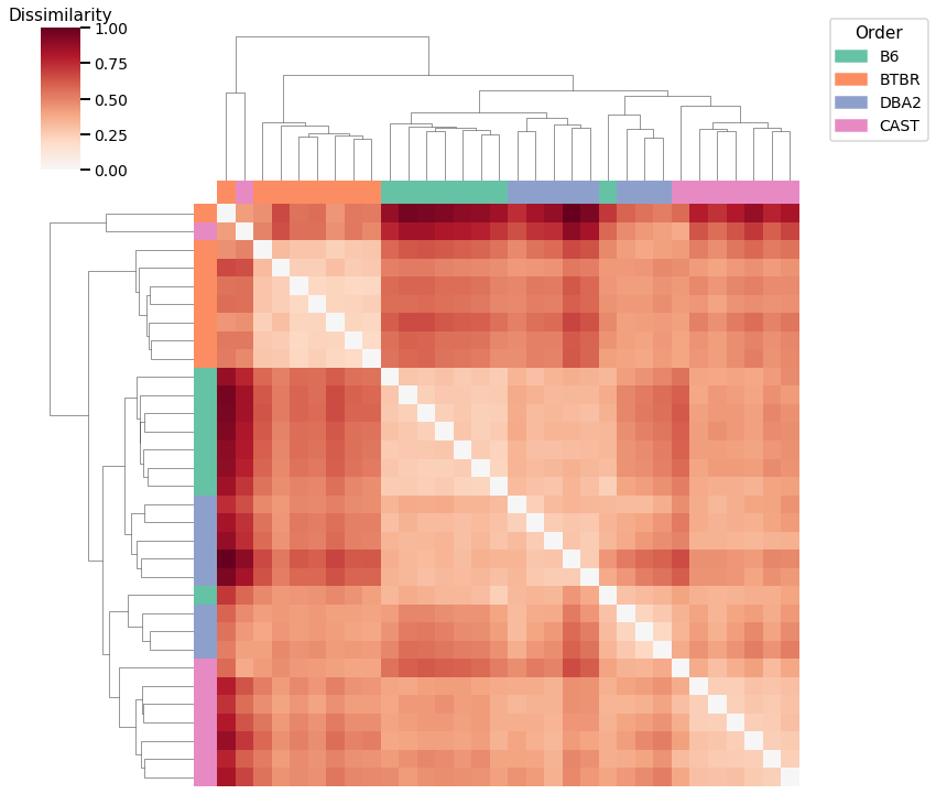
Average of Adjacency Matrix
# HIDE CELL
# calculate dissimilarity matrix
scaled_avgadjmat_dissim = calculate_dissim(graphs, method="avgadjmatrix", norm=None, normalize=True)

# cluster dissimilarity matrix
avgadjmat_linkage_matrix, avgadjmat_pred = cluster_dissim(scaled_avgadjmat_dissim, y, method="agg", n_components=4)

# calculate accuracy and ARI
avgadjmat_pred = remap_labels(y, avgadjmat_pred)
avgadjmat_agg_score = accuracy_score(y, avgadjmat_pred)
avgadjmat_agg_ari = adjusted_rand_score(y, avgadjmat_pred)

print(f"Accuracy: {avgadjmat_agg_score}")
print(f"ARI: {avgadjmat_agg_ari}")

# plot clustered dissimilarity matrix
plot_clustering(labels, 'agg', scaled_avgadjmat_dissim, avgadjmat_linkage_matrix)
Accuracy: 0.65625
ARI: 0.3134054954204829
<seaborn.matrix.ClusterGrid at 0x7fdda190c400>
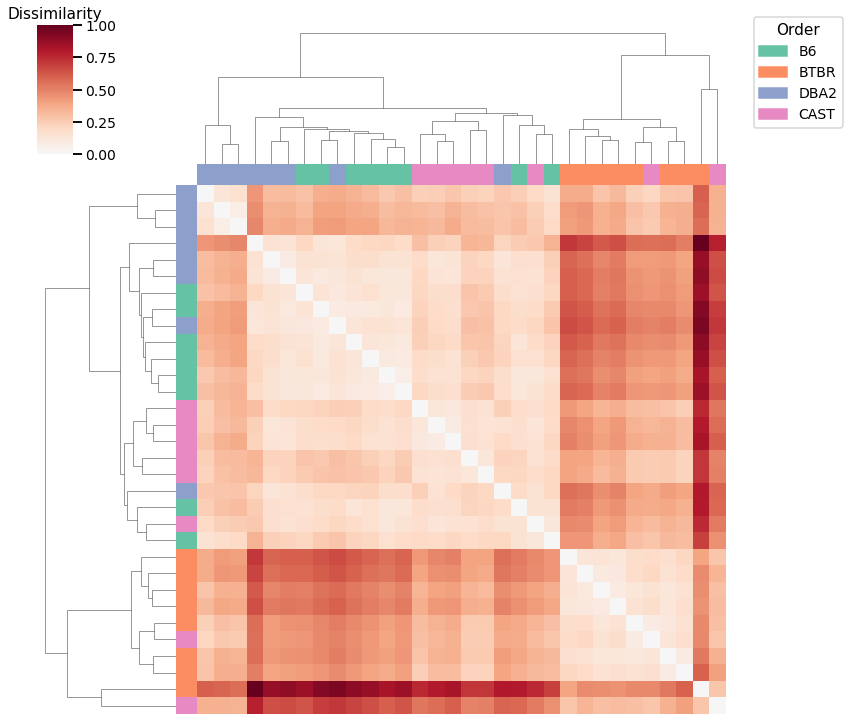
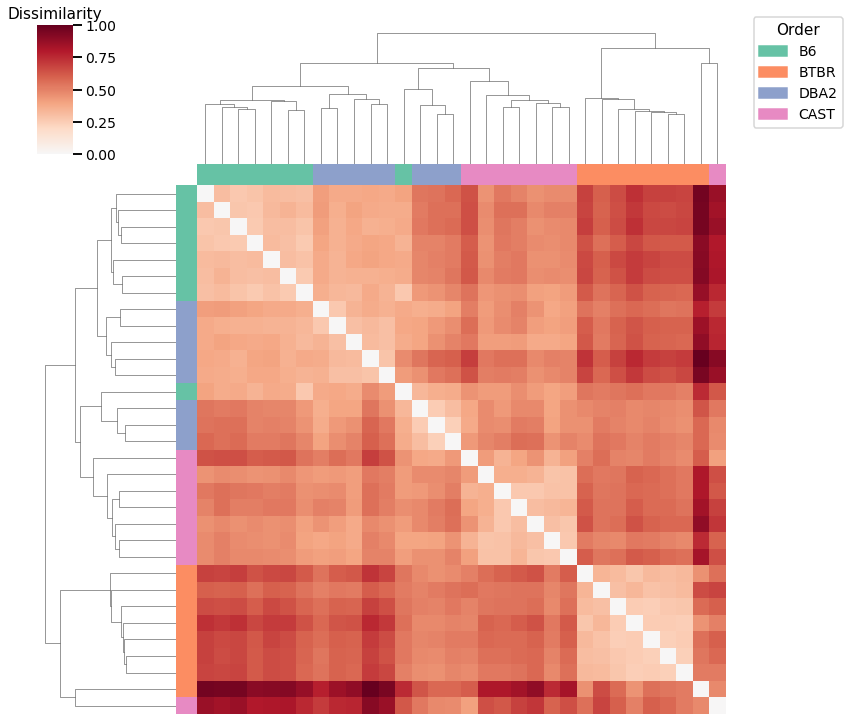
Laplacian Spectral Distance
# HIDE CELL
# calculate dissimilarity matrix
scaled_lap_dissim = laplacian_dissim(graphs, transform='pass-to-ranks', metric='l2', normalize=True)

# cluster dissimilarity matrix
lap_linkage_matrix, lap_pred = cluster_dissim(scaled_lap_dissim, y, method="agg", n_components=4)

# calculate accuracy and ARI
lap_pred = remap_labels(y, lap_pred)
lap_agg_score = accuracy_score(y, lap_pred)
lap_agg_ari = adjusted_rand_score(y, lap_pred)

print(f"Accuracy: {lap_agg_score}")
print(f"ARI: {lap_agg_ari}")

# plot clustered dissimilarity matrix
plot_clustering(labels, 'agg', scaled_lap_dissim, lap_linkage_matrix)
Accuracy: 0.59375
ARI: 0.27906976744186046
<seaborn.matrix.ClusterGrid at 0x7fdd795bbb80>
Node Degrees - L1 Norm
# HIDE CELL
# calculate dissimilarity matrix
scaled_nodedeg_dissim_l1 = calculate_dissim(graphs, method="degree", norm="l1", normalize=True)

# cluster dissimilarity matrix
nodedeg_l1_linkage_matrix, nodedeg_l1_pred = cluster_dissim(scaled_nodedeg_dissim_l1, y, method="agg", n_components=4)

# calculate accuracy and ARI
nodedeg_l1_pred = remap_labels(y, nodedeg_l1_pred)
nodedeg_l1_agg_score = accuracy_score(y, nodedeg_l1_pred)
nodedeg_l1_agg_ari = adjusted_rand_score(y, nodedeg_l1_pred)

print(f"Accuracy: {nodedeg_l1_agg_score}")
print(f"ARI: {nodedeg_l1_agg_ari}")

# plot clustered dissimilarity matrix
plot_clustering(labels, 'agg', scaled_nodedeg_dissim_l1, nodedeg_l1_linkage_matrix)
Accuracy: 0.46875
ARI: 0.17706740792216819
<seaborn.matrix.ClusterGrid at 0x7fdd79524d90>
Node Degrees - L2 Norm
# HIDE CELL
# calculate dissimilarity matrix
scaled_nodedeg_dissim_l2 = calculate_dissim(graphs, method="degree", norm="l2", normalize=True)

# cluster dissimilarity matrix
nodedeg_l2_linkage_matrix, nodedeg_l2_pred = cluster_dissim(scaled_nodedeg_dissim_l2, y, method="agg", n_components=4)

# calculate accuracy and ARI
nodedeg_l2_pred = remap_labels(y, nodedeg_l2_pred)
nodedeg_l2_agg_score = accuracy_score(y, nodedeg_l2_pred)
nodedeg_l2_agg_ari = adjusted_rand_score(y, nodedeg_l2_pred)

print(f"Accuracy: {nodedeg_l2_agg_score}")
print(f"ARI: {nodedeg_l2_agg_ari}")

# plot clustered dissimilarity matrix
plot_clustering(labels, 'agg', scaled_nodedeg_dissim_l2, nodedeg_l2_linkage_matrix)
Accuracy: 0.5
ARI: 0.27552275522755226
<seaborn.matrix.ClusterGrid at 0x7fdd7951c220>
Node Strength - L1 Norm
# HIDE CELL
# calculate dissimilarity matrix
scaled_nodestr_dissim_l1 = calculate_dissim(graphs, method="strength", norm="l1", normalize=True)

# cluster dissimilarity matrix
nodestr_l1_linkage_matrix, nodestr_l1_pred = cluster_dissim(scaled_nodestr_dissim_l1, y, method="agg", n_components=4)

# calculate accuracy and ARI
nodestr_l1_pred = remap_labels(y, nodestr_l1_pred)
nodestr_l1_agg_score = accuracy_score(y, nodestr_l1_pred)
nodestr_l1_agg_ari = adjusted_rand_score(y, nodestr_l1_pred)

print(f"Accuracy: {nodestr_l1_agg_score}")
print(f"ARI: {nodestr_l1_agg_ari}")

# plot clustered dissimilarity matrix
plot_clustering(labels, 'agg', scaled_nodestr_dissim_l1, nodestr_l1_linkage_matrix)
Accuracy: 0.65625
ARI: 0.45908859901744875
<seaborn.matrix.ClusterGrid at 0x7fdda25b3730>
Node Strength - L2 Norm
# HIDE CELL
# calculate dissimilarity matrix
scaled_nodestr_dissim_l2 = calculate_dissim(graphs, method="strength", norm="l2", normalize=True)

# cluster dissimilarity matrix
nodestr_l2_linkage_matrix, nodestr_l2_pred = cluster_dissim(scaled_nodestr_dissim_l2, y, method="agg", n_components=4)

# calculate accuracy and ARI
nodestr_l2_pred = remap_labels(y, nodestr_l2_pred)
nodestr_l2_agg_score = accuracy_score(y, nodestr_l2_pred)
nodestr_l2_agg_ari = adjusted_rand_score(y, nodestr_l2_pred)

print(f"Accuracy: {nodestr_l2_agg_score}")
print(f"ARI: {nodestr_l2_agg_ari}")

# plot clustered dissimilarity matrix
plot_clustering(labels, 'agg', scaled_nodestr_dissim_l2, nodestr_l2_linkage_matrix)
Accuracy: 0.5
ARI: 0.27552275522755226
<seaborn.matrix.ClusterGrid at 0x7fdd87421370>
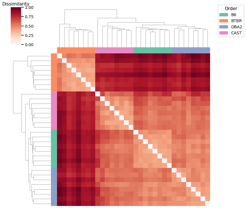
Edge weights - L1 Norm
# HIDE CELL
# calculate dissimilarity matrix
scaled_edgeweight_dissim_l1 = calculate_dissim(graphs, method="edgeweight", norm="l1", normalize=True)

# cluster dissimilarity matrix
edgeweight_l1_linkage_matrix, edgeweight_l1_pred = cluster_dissim(scaled_edgeweight_dissim_l1, y, method="agg", n_components=4)

# calculate accuracy and ARI
edgeweight_l1_pred = remap_labels(y, edgeweight_l1_pred)
edgeweight_l1_agg_score = accuracy_score(y, edgeweight_l1_pred)
edgeweight_l1_agg_ari = adjusted_rand_score(y, edgeweight_l1_pred)

print(f"Accuracy: {edgeweight_l1_agg_score}")
print(f"ARI: {edgeweight_l1_agg_ari}")

# plot clustered dissimilarity matrix
plot_clustering(labels, 'agg', scaled_edgeweight_dissim_l1, edgeweight_l1_linkage_matrix)
Accuracy: 0.6875
ARI: 0.6236421725239617
<seaborn.matrix.ClusterGrid at 0x7fddb1d40550>
Edge weights - L2 Norm
# HIDE CODE
# calculate dissimilarity matrix
scaled_edgeweight_dissim_l2 = calculate_dissim(graphs, method="edgeweight", norm="l2", normalize=True)

# cluster dissimilarity matrix
edgeweight_l2_linkage_matrix, edgeweight_l2_pred = cluster_dissim(scaled_edgeweight_dissim_l2, y, method="agg", n_components=4)

# calculate accuracy and ARI
edgeweight_l2_pred = remap_labels(y, edgeweight_l2_pred)
edgeweight_l2_agg_score = accuracy_score(y, edgeweight_l2_pred)
edgeweight_l2_agg_ari = adjusted_rand_score(y, edgeweight_l2_pred)

print(f"Accuracy: {edgeweight_l2_agg_score}")
print(f"ARI: {edgeweight_l2_agg_ari}")

# plot clustered dissimilarity matrix
plot_clustering(labels, 'agg', scaled_edgeweight_dissim_l2, edgeweight_l2_linkage_matrix)
Accuracy: 0.5
ARI: 0.27552275522755226
<seaborn.matrix.ClusterGrid at 0x7fdda2602c70>
Omnibus Embedding
# HIDE CELL
from graspologic.embed import OmnibusEmbed

# embed using Omni
embedder = OmnibusEmbed(n_elbows=3)
omni_embedding = embedder.fit_transform(graphs)

# calculate dissimilarity matrix
omni_matrix = np.zeros((len(graphs), len(graphs)))
for i, embedding1 in enumerate(omni_embedding):
    for j, embedding2 in enumerate(omni_embedding):
        dist = np.linalg.norm(embedding1 - embedding2, ord="fro")
        omni_matrix[i, j] = dist

scaled_omni_dissim = omni_matrix / np.max(omni_matrix)

# cluster dissimilarity matrix
omni_linkage_matrix, omni_pred = cluster_dissim(scaled_omni_dissim, y, method="agg", n_components=4)

# calculate accuracy and ARI
omni_pred = remap_labels(y, omni_pred)
omni_agg_score = accuracy_score(y, omni_pred)
omni_agg_ari = adjusted_rand_score(y, omni_pred)

print(f"Accuracy: {omni_agg_score}")
print(f"ARI: {omni_agg_ari}")

# plot clustered dissimilarity matrix
plot_clustering(labels, 'agg', scaled_omni_dissim, omni_linkage_matrix)
Accuracy: 0.71875
ARI: 0.6531126871552404
<seaborn.matrix.ClusterGrid at 0x7fdd6034f580>
GMM
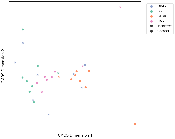
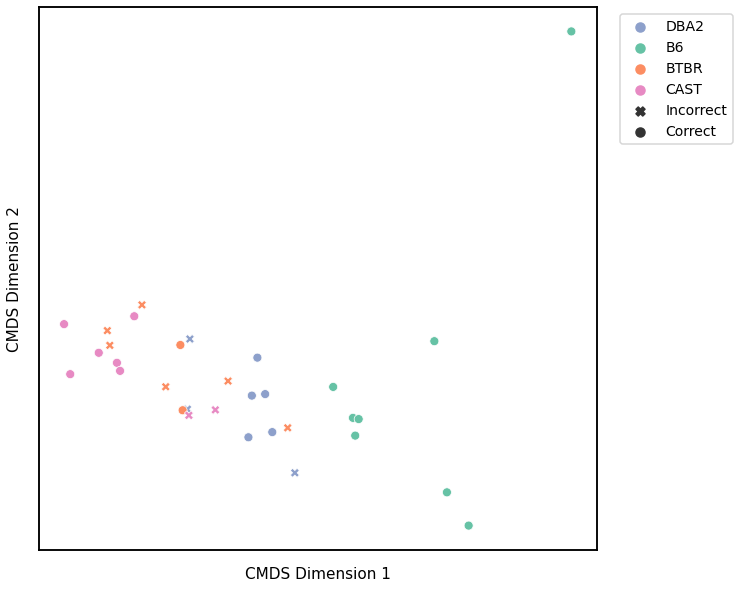
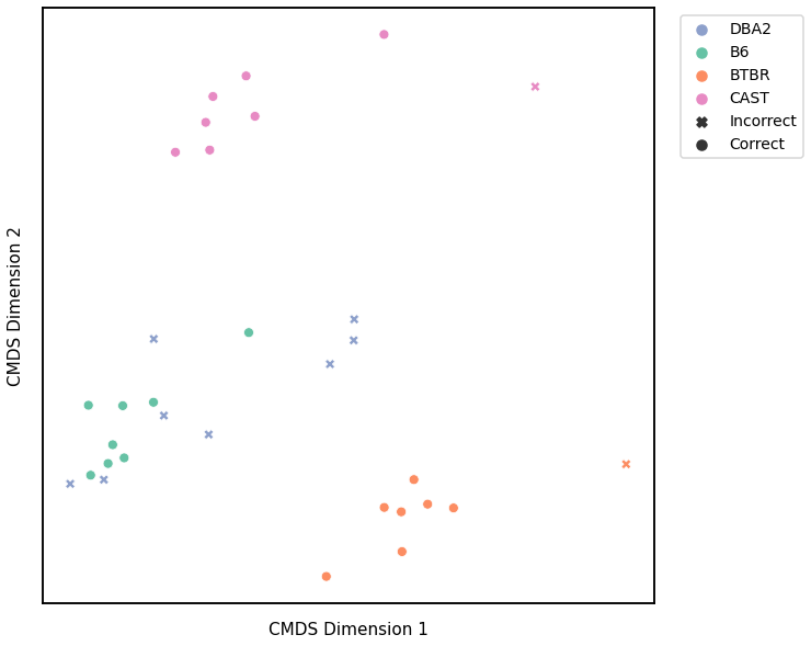
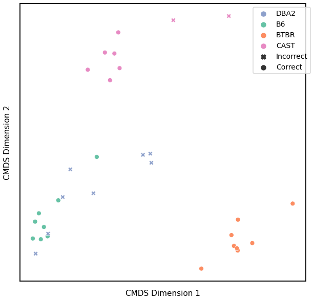
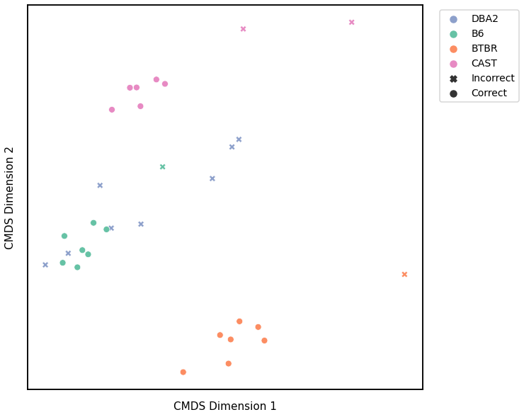
We use classical multidimensional scaling to embed the dissimilarity matrices into a 2-dimensional space, then we use GMM to cluster these points. We assign the number of components to be 4 since there are 4 genotypes, and the clusters are visualized with a scattermap below. The colors indicate the true genotypes, and the shapes (O or X) indicate whether or not the predictions are correct.
For each kernel, we report the accuracy score, the number of correct predictions divided by the total number of samples, and the adjusted rand index.
Density
### HIDE CELL
# cluster dissimilarity matrix
density_gm_embedding, density_gm_pred = cluster_dissim(scaled_density_dissim, y, method='gmm', n_components=4)
density_gm, density_gm_pred = construct_df(density_gm_embedding, labels, y, density_gm_pred)

# calculate accuracy and ARI
density_gm_score = accuracy_score(y, density_gm_pred)
density_gm_ari = adjusted_rand_score(y, density_gm_pred)

print(f"Accuracy: {density_gm_score}")
print(f"ARI: {density_gm_ari}")

# plot clustering
plot_clustering(labels, 'gmm', data=density_gm)
Accuracy: 0.53125
ARI: 0.20111167256189996
<AxesSubplot:xlabel='CMDS Dimension 1', ylabel='CMDS Dimension 2'>
Average Edge Weight
# HIDE CELL
# cluster dissimilarity matrix
avgedgeweight_gm_embedding, avgedgeweight_gm_pred = cluster_dissim(scaled_avgedgeweight_dissim, y, method='gmm', n_components=4)
avgedgeweight_gm, avgedgeweight_gm_pred = construct_df(avgedgeweight_gm_embedding, labels, y, avgedgeweight_gm_pred)

# calculate accuracy and ARI
avgedgeweight_gm_score = accuracy_score(y, avgedgeweight_gm_pred)
avgedgeweight_gm_ari = adjusted_rand_score(y, avgedgeweight_gm_pred)

print(f"Accuracy: {avgedgeweight_gm_score}")
print(f"ARI: {avgedgeweight_gm_ari}")

# plot clustering
plot_clustering(labels, 'gmm', data=avgedgeweight_gm)
Accuracy: 0.65625
ARI: 0.39636032757051864
<AxesSubplot:xlabel='CMDS Dimension 1', ylabel='CMDS Dimension 2'>
Average of the Adjacency Matrix
# HIDE CELL
# cluster dissimilarity matrix
avgadjmat_gm_embedding, avgadjmat_gm_pred = cluster_dissim(scaled_avgadjmat_dissim, y, method="gmm", n_components=4)
avgadjmat_gm, avgadjmat_gm_pred = construct_df(avgadjmat_gm_embedding, labels, y, avgadjmat_gm_pred)

# calculate accuracy and ARI
avgadjmat_gm_score = accuracy_score(y, avgadjmat_gm_pred)
avgadjmat_gm_ari = adjusted_rand_score(y, avgadjmat_gm_pred)

print(f"Accuracy: {avgadjmat_gm_score}")
print(f"ARI: {avgadjmat_gm_ari}")

# plot clustering
plot_clustering(labels, 'gmm', data=avgadjmat_gm)
Accuracy: 0.59375
ARI: 0.27401624980086026
<AxesSubplot:xlabel='CMDS Dimension 1', ylabel='CMDS Dimension 2'>
Laplacian Spectral Distance
# HIDE CELL
# cluster dissimilarity matrix
lap_gm_embedding, lap_gm_pred = cluster_dissim(scaled_lap_dissim, y, method="gmm", n_components=4)
lap_gm, lap_gm_pred = construct_df(lap_gm_embedding, labels, y, lap_gm_pred)

# calculate accuracy and ARI
lap_gm_score = accuracy_score(y, lap_gm_pred)
lap_gm_ari = adjusted_rand_score(y, lap_gm_pred)

print(f"Accuracy: {lap_gm_score}")
print(f"ARI: {lap_gm_ari}")

# plot clustering
plot_clustering(labels, 'gmm', data=lap_gm)
Accuracy: 0.5625
ARI: 0.29275603663613653
<AxesSubplot:xlabel='CMDS Dimension 1', ylabel='CMDS Dimension 2'>
Node Degrees - L1 Norm
# HIDE CELL
# cluster dissimilarity matrix
nodedeg_l1_gm_embedding, nodedeg_l1_gm_pred = cluster_dissim(scaled_nodedeg_dissim_l1, y, method="gmm", n_components=4)
nodedeg_l1_gm, nodedeg_l1_gm_pred = construct_df(nodedeg_l1_gm_embedding, labels, y, nodedeg_l1_gm_pred)

# calculate accuracy and ARI
nodedeg_l1_gm_score = accuracy_score(y, nodedeg_l1_gm_pred)
nodedeg_l1_gm_ari = adjusted_rand_score(y, nodedeg_l1_gm_pred)

print(f"Accuracy: {nodedeg_l1_gm_score}")
print(f"ARI: {nodedeg_l1_gm_ari}")

# plot clustering
fig = plot_clustering(labels, 'gmm', data=nodedeg_l1_gm)
fig.legend(bbox_to_anchor=(1.257, 1))
Accuracy: 0.78125
ARI: 0.5656050955414013
<matplotlib.legend.Legend at 0x7fdda7ef05b0>
Node Degrees - L2 Norm
# HIDE CELL
# cluster dissimilarity matrix
nodedeg_l2_gm_embedding, nodedeg_l2_gm_pred = cluster_dissim(scaled_nodedeg_dissim_l2, y, method="gmm", n_components=4)
nodedeg_l2_gm, nodedeg_l2_gm_pred = construct_df(nodedeg_l2_gm_embedding, labels, y, nodedeg_l2_gm_pred)

# calculate accuracy and ARI
nodedeg_l2_gm_score = accuracy_score(y, nodedeg_l2_gm_pred)
nodedeg_l2_gm_ari = adjusted_rand_score(y, nodedeg_l2_gm_pred)

print(f"Accuracy: {nodedeg_l2_gm_score}")
print(f"ARI: {nodedeg_l2_gm_ari}")

# plot clustering
fig = plot_clustering(labels, 'gmm', data=nodedeg_l2_gm)
fig.legend(bbox_to_anchor=(1.257, 1))
Accuracy: 0.6875
ARI: 0.5248441974060973
<matplotlib.legend.Legend at 0x7fdd6074dcd0>
Node Strength - L1 Norm
# HIDE CELL
# cluster dissimilarity matrix
nodestr_l1_gm_embedding, nodestr_l1_gm_pred = cluster_dissim(scaled_nodestr_dissim_l1, y, method="gmm", n_components=4)
nodestr_l1_gm, nodestr_l1_gm_pred = construct_df(nodestr_l1_gm_embedding, labels, y, nodestr_l1_gm_pred)

# calculate accuracy and ARI
nodestr_l1_gm_score = accuracy_score(y, nodestr_l1_gm_pred)
nodestr_l1_gm_ari = adjusted_rand_score(y, nodestr_l1_gm_pred)

print(f"Accuracy: {nodestr_l1_gm_score}")
print(f"ARI: {nodestr_l1_gm_ari}")

# plot clustering
fig = plot_clustering(labels, 'gmm', data=nodestr_l1_gm)
fig.legend(bbox_to_anchor=(1.257, 1))
Accuracy: 0.65625
ARI: 0.45908859901744875
<matplotlib.legend.Legend at 0x7fdd7b858760>
Node Strength - L2 Norm
# HIDE CELL
# cluster dissimilarity matrix
nodestr_l2_gm_embedding, nodestr_l2_gm_pred = cluster_dissim(scaled_nodestr_dissim_l2, y, method="gmm", n_components=4)
nodestr_l2_gm, nodestr_l2_gm_pred = construct_df(nodestr_l2_gm_embedding, labels, y, nodestr_l2_gm_pred)

# calculate accuracy and ARI
nodestr_l2_gm_score = accuracy_score(y, nodestr_l2_gm_pred)
nodestr_l2_gm_ari = adjusted_rand_score(y, nodestr_l2_gm_pred)

print(f"Accuracy: {nodestr_l2_gm_score}")
print(f"ARI: {nodestr_l2_gm_ari}")

# plot clustering
fig = plot_clustering(labels, 'gmm', data=nodestr_l2_gm)
fig.legend(bbox_to_anchor=(1.257, 1))
Accuracy: 0.6875
ARI: 0.5536168050143995
<matplotlib.legend.Legend at 0x7fdd913d3910>
Edge Weights - L1 Norm
# HIDE CELL
# cluster dissimilarity matrix
edgeweight_l1_gm_embedding, edgeweight_l1_gm_pred = cluster_dissim(scaled_edgeweight_dissim_l1, y, method="gmm", n_components=4)
edgeweight_l1_gm, edgeweight_l1_gm_pred = construct_df(edgeweight_l1_gm_embedding, labels, y, edgeweight_l1_gm_pred)

# calculate accuracy and ARI
edgeweight_l1_gm_score = accuracy_score(y, edgeweight_l1_gm_pred)
edgeweight_l1_gm_ari = adjusted_rand_score(y, edgeweight_l1_gm_pred)

print(f"Accuracy: {edgeweight_l1_gm_score}")
print(f"ARI: {edgeweight_l1_gm_ari}")

# plot clustering
fig = plot_clustering(labels, 'gmm', data=edgeweight_l1_gm)
fig.legend(bbox_to_anchor=(1.257, 1))
Accuracy: 0.71875
ARI: 0.6531126871552404
<matplotlib.legend.Legend at 0x7fdda6fbdc70>
Edge Weights - L2 Norm
# HIDE CELL
from graspologic.utils import symmetrize

# make dissimilarity matrix symmetric
scaled_edgeweight_dissim_l2 = symmetrize(scaled_edgeweight_dissim_l2)

# cluster dissimilarity matrix
edgeweight_l2_gm_embedding, edgeweight_l2_gm_pred = cluster_dissim(dissim_matrix=scaled_edgeweight_dissim_l2, labels=y, \
    method="gmm", n_components=4)
edgeweight_l2_gm, edgeweight_l2_gm_pred = construct_df(edgeweight_l2_gm_embedding, labels, y, edgeweight_l2_gm_pred)

# calculate accuracy and ARI
edgeweight_l2_gm_score = accuracy_score(y, edgeweight_l2_gm_pred)
edgeweight_l2_gm_ari = adjusted_rand_score(y, edgeweight_l2_gm_pred)

print(f"Accuracy: {edgeweight_l2_gm_score}")
print(f"ARI: {edgeweight_l2_gm_ari}")

# plot clustering
fig = plot_clustering(labels, 'gmm', data=edgeweight_l2_gm)
Accuracy: 0.6875
ARI: 0.5536168050143995
Omnibus Embedding
# HIDE CELL
# cluster dissimilarity matrix
omni_gm_embedding, omni_gm_pred = cluster_dissim(scaled_omni_dissim, y, method="gmm", n_components=4)
omni_gm, omni_gm_pred = construct_df(omni_gm_embedding, labels, y, omni_gm_pred)

# calculate accuracy and ARI
omni_gm_score = accuracy_score(y, omni_gm_pred)
omni_gm_ari = adjusted_rand_score(y, omni_gm_pred)

print(f"Accuracy: {omni_gm_score}")
print(f"ARI: {omni_gm_ari}")

# plot clustering
fig = plot_clustering(labels, 'gmm', data=omni_gm)
fig.legend(bbox_to_anchor=(1.257, 1))
Accuracy: 0.84375
ARI: 0.6916259721468621
<matplotlib.legend.Legend at 0x7fdd913f4e50>
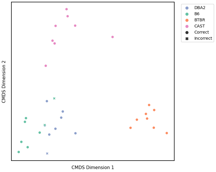
KMeans
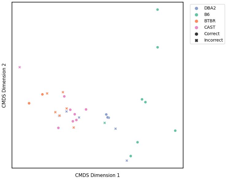
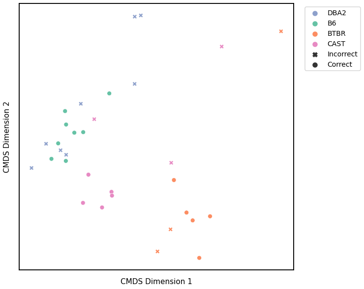
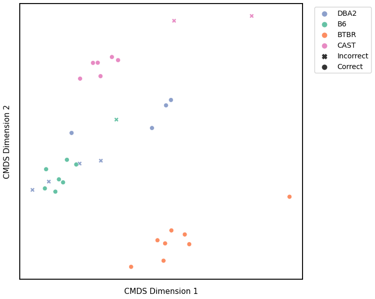
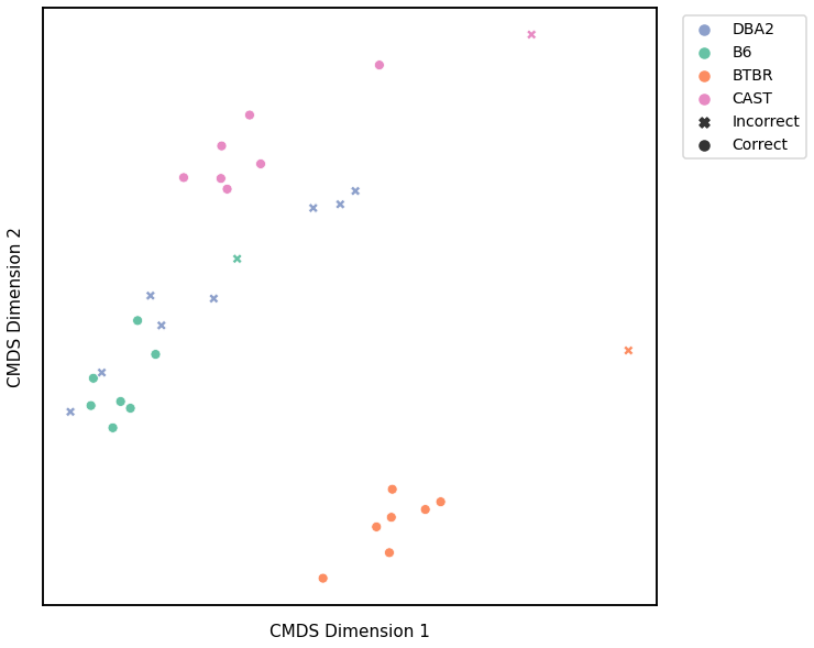
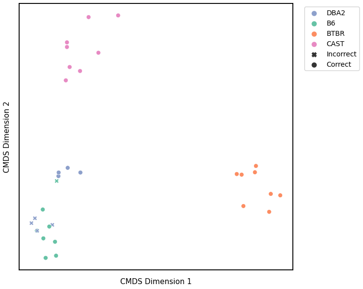
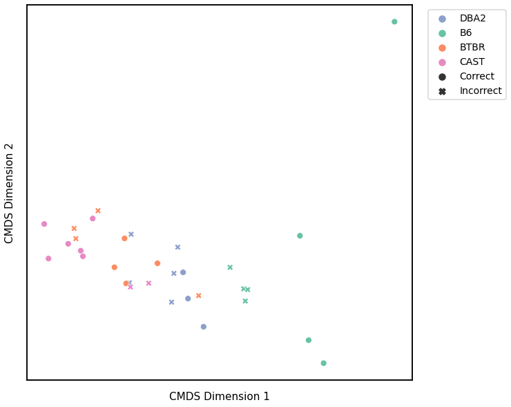
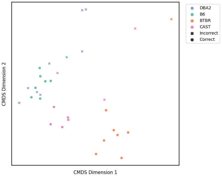
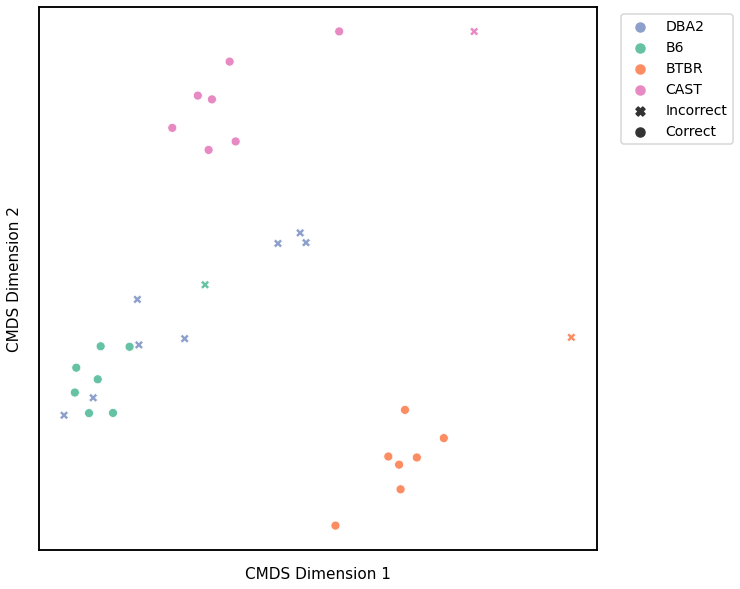
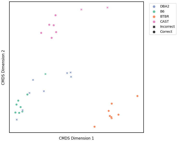
Similar to GMM, we first use classical multidimensional scaling to embed the dissimilarity matrices into a 2-dimensional space, then use KMeans to predict the genotypes of each point. The clusters are shown in the scatterplot below, and the colors represent the true genotypes and the shapes (O or X) indicate whether or not we made correct predictions.
For each kernel, we report the raw accuracy score, the number of correct predictions divided by the total number of samples, and the adjusted rand index.
Density
# HIDE CELL
# cluster dissimilarity matrix
density_km_embedding, density_km_pred = cluster_dissim(scaled_density_dissim, y, method="kmeans", n_components=4)
density_km, density_km_pred = construct_df(density_km_embedding, labels, y, density_km_pred)

# calculate accuracy and ARI
density_km_score = accuracy_score(y, density_km_pred)
density_km_ari = adjusted_rand_score(y, density_km_pred)

print(f"Accuracy: {density_km_score}")
print(f"ARI: {density_km_ari}")

# plot clustering
plot_clustering(labels, 'kmeans', data=density_km)
Accuracy: 0.5625
ARI: 0.24777853725222146
<AxesSubplot:xlabel='CMDS Dimension 1', ylabel='CMDS Dimension 2'>

Average Edge Weight
# HIDE CELL
# cluster dissimilarity matrix
avgedgeweight_km_embedding, avgedgeweight_km_pred = cluster_dissim(scaled_avgedgeweight_dissim, y, method='kmeans', n_components=4)
avgedgeweight_km, avgedgeweight_km_pred = construct_df(avgedgeweight_km_embedding, labels, y, avgedgeweight_km_pred)

# calculate accuracy and ARI
avgedgeweight_km_score = accuracy_score(y, avgedgeweight_km_pred)
avgedgeweight_km_ari = adjusted_rand_score(y, avgedgeweight_km_pred)

print(f"Accuracy: {avgedgeweight_km_score}")
print(f"ARI: {avgedgeweight_km_ari}")

# plot clustering
plot_clustering(labels, 'kmeans', data=avgedgeweight_km)
Accuracy: 0.53125
ARI: 0.2412006432017152
<AxesSubplot:xlabel='CMDS Dimension 1', ylabel='CMDS Dimension 2'>
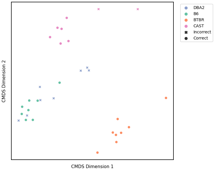
Average of the Adjacency Matrix
# HIDE CELL
# cluster dissimilarity matrix
avgadjmat_km_embedding, avgadjmat_km_pred = cluster_dissim(scaled_avgadjmat_dissim, y, method='kmeans', n_components=4)
avgadjmat_km, avgadjmat_km_pred = construct_df(avgadjmat_km_embedding, labels, y, avgadjmat_km_pred)

# calculate accuracy and ARI
avgadjmat_km_score = accuracy_score(y, avgadjmat_km_pred)
avgadjmat_km_ari = adjusted_rand_score(y, avgadjmat_km_pred)

print(f"Accuracy: {avgadjmat_km_score}")
print(f"ARI: {avgadjmat_km_ari}")

# plot clustering
plot_clustering(labels, 'kmeans', data=avgadjmat_km)
Accuracy: 0.65625
ARI: 0.3094958968347011
<AxesSubplot:xlabel='CMDS Dimension 1', ylabel='CMDS Dimension 2'>

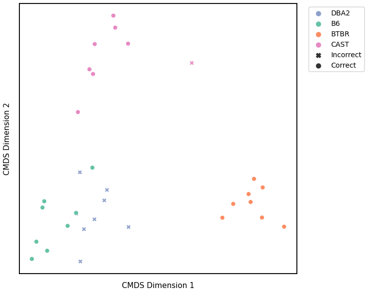
Laplacian Spectral Distance
# HIDE CELL
# cluster dissimilarity matrix
lap_km_embedding, lap_km_pred = cluster_dissim(scaled_lap_dissim, y, method="gmm", n_components=4)
lap_km, lap_km_pred = construct_df(lap_km_embedding, labels, y, lap_km_pred)

# calculate accuracy and ARI
lap_km_score = accuracy_score(y, lap_km_pred)
lap_km_ari = adjusted_rand_score(y, lap_km_pred)

print(f"Accuracy: {lap_km_score}")
print(f"ARI: {lap_km_ari}")

# plot clustering
plot_clustering(labels, 'gmm', data=lap_km)
Accuracy: 0.59375
ARI: 0.34355412502117566
<AxesSubplot:xlabel='CMDS Dimension 1', ylabel='CMDS Dimension 2'>
Node Degree - L1 Norm
# HIDE CELL
# cluster dissimilarity matrix
nodedeg_l1_km_embedding, nodedeg_l1_km_pred = cluster_dissim(scaled_nodedeg_dissim_l1, y, method='kmeans', n_components=4)
nodedeg_l1_km, nodedeg_l1_km_pred = construct_df(nodedeg_l1_km_embedding, labels, y, nodedeg_l1_km_pred)

# calculate accuracy and ARI
nodedeg_l1_km_score = accuracy_score(y, nodedeg_l1_km_pred)
nodedeg_l1_km_ari = adjusted_rand_score(y, nodedeg_l1_km_pred)

print(f"Accuracy: {nodedeg_l1_km_score}")
print(f"ARI: {nodedeg_l1_km_ari}")

# plot clustering
fig = plot_clustering(labels, 'kmeans', data=nodedeg_l1_km)
fig.legend(bbox_to_anchor=(1.257, 1))
Accuracy: 0.625
ARI: 0.36778063410454154
<matplotlib.legend.Legend at 0x7fdda67c5490>
Node Degree - L2 Norm
# HIDE CELL
# cluster dissimilarity matrix
nodedeg_l2_km_embedding, nodedeg_l2_km_pred = cluster_dissim(scaled_nodedeg_dissim_l2, y, method='kmeans', n_components=4)
nodedeg_l2_km, nodedeg_l2_km_pred = construct_df(nodedeg_l2_km_embedding, labels, y, nodedeg_l2_km_pred)

# calculate accuracy and ARI
nodedeg_l2_km_score = accuracy_score(y, nodedeg_l2_km_pred)
nodedeg_l2_km_ari = adjusted_rand_score(y, nodedeg_l2_km_pred)

print(f"Accuracy: {nodedeg_l2_km_score}")
print(f"ARI: {nodedeg_l2_km_ari}")

# plot clustering
fig = plot_clustering(labels, 'kmeans', data=nodedeg_l2_km)
fig.legend(bbox_to_anchor=(1.257, 1))
Accuracy: 0.65625
ARI: 0.47026657552973344
<matplotlib.legend.Legend at 0x7fddb43686d0>

Node Strength - L1 Norm
# HIDE CELL
# cluster dissimilarity matrix
nodestr_l1_km_embedding, nodestr_l1_km_pred = cluster_dissim(scaled_nodestr_dissim_l1, y, method='kmeans', n_components=4)
nodestr_l1_km, nodestr_l1_km_pred = construct_df(nodestr_l1_km_embedding, labels, y, nodestr_l1_km_pred)

# calculate accuracy and ARI
nodestr_l1_km_score = accuracy_score(y, nodestr_l1_km_pred)
nodestr_l1_km_ari = adjusted_rand_score(y, nodestr_l1_km_pred)

print(f"Accuracy: {nodestr_l1_km_score}")
print(f"ARI: {nodestr_l1_km_ari}")

# plot clustering
fig = plot_clustering(labels, 'kmeans', data=nodestr_l1_km)
fig.legend(bbox_to_anchor=(1.257, 1))
Accuracy: 0.65625
ARI: 0.44858546501778757
<matplotlib.legend.Legend at 0x7fdd7931ed00>

Node Strength - L2 Norm
# HIDE CELL
# cluster dissimilarity matrix
nodestr_l2_km_embedding, nodestr_l2_km_pred = cluster_dissim(scaled_nodestr_dissim_l2, y, method='kmeans', n_components=4)
nodestr_l2_km, nodestr_l2_km_pred = construct_df(nodestr_l2_km_embedding, labels, y, nodestr_l2_km_pred)

# calculate accuracy and ARI
nodestr_l2_km_score = accuracy_score(y, nodestr_l2_km_pred)
nodestr_l2_km_ari = adjusted_rand_score(y, nodestr_l2_km_pred)

print(f"Accuracy: {nodestr_l2_km_score}")
print(f"ARI: {nodestr_l2_km_ari}")

# plot clustering
fig = plot_clustering(labels, 'kmeans', data=nodestr_l2_km)
fig.legend(bbox_to_anchor=(1.257, 1))
Accuracy: 0.65625
ARI: 0.45908859901744875
<matplotlib.legend.Legend at 0x7fddb488caf0>
Edge Weight - L1 Norm
# HIDE CELL
# cluster dissimilarity matrix
edgeweight_l1_km_embedding, edgeweight_l1_km_pred = cluster_dissim(scaled_edgeweight_dissim_l1, y, method='kmeans', n_components=4)
edgeweight_l1_km, edgeweight_l1_km_pred = construct_df(edgeweight_l1_km_embedding, labels, y, edgeweight_l1_km_pred)

# calculate accuracy and ARI
edgeweight_l1_km_score = accuracy_score(y, edgeweight_l1_km_pred)
edgeweight_l1_km_ari = adjusted_rand_score(y, edgeweight_l1_km_pred)

print(f"Accuracy: {edgeweight_l1_km_score}")
print(f"ARI: {edgeweight_l1_km_ari}")

# plot clustering
fig = plot_clustering(labels, 'kmeans', data=edgeweight_l1_km)
fig.legend(bbox_to_anchor=(1.257, 1))
Accuracy: 0.90625
ARI: 0.7758205080660115
<matplotlib.legend.Legend at 0x7fdda29d8dc0>
Edge Weight - L2 Norm
# HIDE CELL
# cluster dissimilarity matrix
edgeweight_l2_km_embedding, edgeweight_l2_km_pred = cluster_dissim(scaled_edgeweight_dissim_l2, y, method='kmeans', n_components=4)
edgeweight_l2_km, edgeweight_l2_km_pred = construct_df(edgeweight_l2_km_embedding, labels, y, edgeweight_l2_km_pred)

# calculate accuracy and ARI
edgeweight_l2_km_score = accuracy_score(y, edgeweight_l2_km_pred)
edgeweight_l2_km_ari = adjusted_rand_score(y, edgeweight_l2_km_pred)

print(f"Accuracy: {edgeweight_l2_km_score}")
print(f"ARI: {edgeweight_l2_km_ari}")

# plot clustering
fig = plot_clustering(labels, 'kmeans', data=edgeweight_l2_km)
fig.legend(bbox_to_anchor=(1.257, 1))
Accuracy: 0.65625
ARI: 0.4914559125085441
<matplotlib.legend.Legend at 0x7fdd71f40580>
Omnibus Embedding
# HIDE CELL
# cluster dissimilarity matrix
omni_km_embedding, omni_km_pred = cluster_dissim(scaled_omni_dissim, y, method='kmeans', n_components=4)
omni_km, omni_km_pred = construct_df(omni_km_embedding, labels, y, omni_km_pred)

# calculate accuracy and ARI
omni_km_score = accuracy_score(y, omni_km_pred)
omni_km_ari = adjusted_rand_score(y, omni_km_pred)

print(f"Accuracy: {omni_km_score}")
print(f"ARI: {omni_km_ari}")

# plot clustering
fig = plot_clustering(labels, 'kmeans', data=omni_km)
fig.legend(bbox_to_anchor=(1.257, 1))
Accuracy: 0.84375
ARI: 0.6916259721468621
<matplotlib.legend.Legend at 0x7fdd7951c4f0>

ARI Plot
We use the adjusted rand index (ARI) to compare the performace of each clustering algorithm on each kernel. The ARI values are visualized with a scatter plot below, and the colors represent the different clustering algorithms. The kernels are sorted by the average ARI value of the three clustering algorithms, from highest to lowest. We also compute the ARI values for each clustering algorithm for a random matrix, which is indicated by the red dash line and should be close to 0.
# HIDE CODE
# construct symmetric random matrix with zero diagonal
np.random.seed(3)
scaled_random = np.random.rand(len(graphs), len(graphs))
scaled_random = symmetrize(scaled_random)

# agglomerative clustering
random_linkage_matrix, random_pred = cluster_dissim(scaled_random, y, method="agg", n_components=4)
random_pred = remap_labels(y, random_pred)
random_agg_score = accuracy_score(y, random_pred)
random_agg_ari = adjusted_rand_score(y, random_pred)

# GMM
random_gm_embedding, random_gm_pred = cluster_dissim(scaled_random, y, method="gmm", n_components=4)
random_gm, random_gm_pred = construct_df(random_gm_embedding, labels, y, random_gm_pred)
random_gm_score = accuracy_score(y, random_gm_pred)
random_gm_ari = adjusted_rand_score(y, random_gm_pred)

# KMeans
random_km_embedding, random_km_pred = cluster_dissim(scaled_random, y, method="kmeans", n_components=4)
random_km, random_km_pred = construct_df(random_km_embedding, labels, y, random_km_pred)
random_km_score = accuracy_score(y, random_km_pred)
random_km_ari = adjusted_rand_score(y, random_km_pred)

random_avg_ari_val = (random_agg_ari + random_gm_ari + random_km_ari) / 3
# HIDE CODE
from matplotlib.patches import Patch

kernels = ['Omnibus', 'Density', 'Avg. Edge Weight', 'Avg. Adj.', 'Laplacian', 'Node Degree (L1)', 'Node Degree (L2)', \
    'Node Strength (L1)', 'Node Strength (L2)', 'Edge Weight (L1)', 'Edge Weight (L2)']
kernels_df = [kernel for kernel in kernels for i in range(3)]
agg_ari = [omni_agg_ari, density_agg_ari, avgedgeweight_agg_ari, avgadjmat_agg_ari, lap_agg_ari, nodedeg_l1_agg_ari, \
    nodedeg_l2_agg_ari, nodestr_l1_agg_ari, nodestr_l2_agg_ari, edgeweight_l1_agg_ari, edgeweight_l2_agg_ari]
gm_ari = [omni_gm_ari, density_gm_ari, avgedgeweight_gm_ari, avgadjmat_gm_ari, lap_gm_ari, nodedeg_l1_gm_ari, \
    nodedeg_l2_gm_ari, nodestr_l1_gm_ari, nodestr_l2_gm_ari, edgeweight_l1_gm_ari, edgeweight_l2_gm_ari]
km_ari = [omni_km_ari, density_km_ari, avgedgeweight_km_ari, avgadjmat_km_ari, lap_km_ari, nodedeg_l1_km_ari, \
    nodedeg_l2_km_ari, nodestr_l1_km_ari, nodestr_l2_km_ari, edgeweight_l1_km_ari, edgeweight_l2_km_ari]

ari_vals = np.vstack((np.array(agg_ari), np.array(gm_ari), np.array(km_ari)))
ari_vals = np.ravel(ari_vals.T)
algos = ['Agglomerative', 'GMM', 'KMeans'] * len(agg_ari)

ari_df = pd.DataFrame(list(zip(kernels_df, ari_vals, algos)), columns=["Kernel", "ARI", "Algorithm"])

avg_ari_vals = (np.array(agg_ari) + np.array(gm_ari) + np.array(km_ari)) / 3
avg_ari_vals = [val for val in avg_ari_vals for i in range(3)]
ari_df["Average"] = avg_ari_vals
ari_df = ari_df.sort_values(by=['Average'], ascending=False)

ari_palette = {'KMeans': list(sns.color_palette())[0], 'GMM': list(sns.color_palette())[1], \
    'Agglomerative': list(sns.color_palette())[2]}
#patches = [Patch(color=v, label=k) for k,v in ari_palette.items()]

mice_cluster_fig, ax = plt.subplots(figsize=(14, 8), facecolor='w')
sns.set_context("talk", font_scale=0.9)
sns.scatterplot(x="Kernel", y="ARI", hue="Algorithm", data=ari_df, alpha=0.6, s=150, palette=ari_palette)
plt.axhline(y=random_avg_ari_val, color='r', linestyle='--', linewidth=2, label='Random')
plt.legend()
plt.xticks(rotation=45)
plt.grid(linewidth=0.5)

glue("mice_cluster", mice_cluster_fig, display=False)
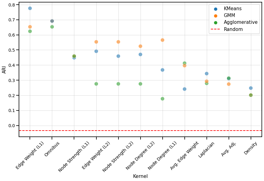
Fig. 5 Scatter plot comparing the ARI values of each clustering algorithm for every kernel, from highest to lowest based on the average ARI value. All kernels perform better than chance.
We observe that the Edge weight kernel (\(L^1\)-norm) performs the best overall. Similar to that of the discriminability plot, kernels that use node matching perform better than those based on global properties, including the Laplacian spectral kernel. The order of the kernels in the ARI plot seem to follow a similar order of that in the discriminability plot for matched networks, which suggests that the dissimilarity matrix may influence their performance more than the choice in clustering algorithm. However, GMM does perform consistently well, either having the highest or middle ARI value for every kernel.