Note
Go to the end to download the full example code
Co-MIGHT when Data Exhibits Conditional Independence#
In this example, we demonstrate how to test the conditional mutual information (CMI) hypothesis test using conditional mutual information for genuine hypothesis test (Co-MIGHT). To perform CMI testing, we have the hypothesis test:
$H_0: I(X_2; Y | X_1) = 0$
$H_1: I(X_2; Y | X_1) > 0$
Here, we simulate two feature-sets, which follow the null-hypothesis with the specific setting that $X_2 perp {Y, X_1}$. We will test using the multi-view decision tree to verify that that the null hypothesis is not rejected.
import matplotlib.pyplot as plt
import numpy as np
from sklearn.datasets import make_classification

from sktree import HonestForestClassifier
from sktree.stats import FeatureImportanceForestClassifier
from sktree.tree import DecisionTreeClassifier, MultiViewDecisionTreeClassifier

seed = 12345
rng = np.random.default_rng(seed)
Simulate data#
We simulate the two feature sets, and the target variable. We then combine them into a single dataset to perform hypothesis testing.
n_samples = 200
n_features_1 = 20
noise_dims = 80
n_features_2 = 1000

signal_X, y = make_classification(
    n_samples=n_samples,
    n_features=n_features_1 + noise_dims,
    n_informative=n_features_1,
    n_redundant=50,
    n_repeated=0,
    n_classes=2,
    class_sep=0.5,
    flip_y=0.01,
    shuffle=True,
    random_state=seed,
)

# model parameters
n_estimators = 200
max_features = 0.3
test_size = 0.2
n_repeats = 1000
n_jobs = -1
Analysis when the null hypothesis is true#
Let’s now investigate what happens when the null hypothesis is true. We will simulate data from the graphical model:
$(X_1 \rightarrow Y; X_2)$
Here, we either have $X_1$ or $X_2$ informative for the target, but not both. We will then perform hypothesis testing using the same procedure as above. We will test the settings when the high-dimensional feature-set is informative for the target, and when the low-dimensional feature-set is informative for the target.
# Make X_2 high-dimensional
n_features_ends = [n_features_1 + noise_dims, signal_X.shape[1]]
_X = np.hstack((signal_X, rng.standard_normal(size=(n_samples, n_features_2))))
X = _X.copy()
n_features_ends[1] = X.shape[1]

print(X.shape, y.shape, n_features_ends)

est = FeatureImportanceForestClassifier(
    estimator=HonestForestClassifier(
        n_estimators=n_estimators,
        max_features=max_features,
        tree_estimator=MultiViewDecisionTreeClassifier(
            feature_set_ends=n_features_ends,
            apply_max_features_per_feature_set=True,
        ),
        random_state=seed,
        honest_fraction=0.5,
        n_jobs=n_jobs,
    ),
    random_state=seed,
    test_size=test_size,
    sample_dataset_per_tree=False,
)

rf_est = FeatureImportanceForestClassifier(
    estimator=HonestForestClassifier(
        n_estimators=n_estimators,
        max_features=max_features,
        tree_estimator=DecisionTreeClassifier(),
        random_state=seed,
        honest_fraction=0.5,
        n_jobs=n_jobs,
    ),
    random_state=seed,
    test_size=test_size,
)

rf_results = dict()
mv_results = dict()

# we test for the first feature set, which is lower-dimensional
covariate_index = np.arange(n_features_ends[0], dtype=int)
stat, pvalue = est.test(X, y, covariate_index=covariate_index, metric="mi", n_repeats=n_repeats)

mv_results["low_dim_feature_stat"] = stat
mv_results["low_dim_feature_pvalue"] = pvalue
print("\n\nImportant feature-set is low-dimensional")
print(f"Estimated MI difference with first view (has dependency): {stat} with Pvalue: {pvalue}")

# we test for the second feature set, which is higher-dimensional
covariate_index = np.arange(n_features_ends[0], n_features_ends[1], dtype=int)
stat, pvalue = est.test(
    X,
    y,
    covariate_index=covariate_index,
    metric="mi",
    n_repeats=n_repeats,
)
mv_results["high_dim_feature_stat"] = stat
mv_results["high_dim_feature_pvalue"] = pvalue
print(
    f"Estimated MI difference testing second view (does not have dependency): "
    f"{stat} with Pvalue: {pvalue}"
)
(200, 1100) (200,) [100, 1100]


Important feature-set is low-dimensional
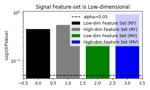
Estimated MI difference with first view (has dependency): -0.000531159335617648 with Pvalue: 0.23676323676323677
Estimated MI difference testing second view (does not have dependency): 9.621981566387827e-05 with Pvalue: 0.916083916083916
Now, we will compare with using a standard decision tree classifier as our base model.
covariate_index = np.arange(n_features_ends[0], dtype=int)
stat, pvalue = rf_est.test(X, y, covariate_index=covariate_index, metric="mi", n_repeats=n_repeats)

rf_results["low_dim_feature_stat"] = stat
rf_results["low_dim_feature_pvalue"] = pvalue
print("\n\nComparing with random forest.")
print(f"Estimated MI difference with first view (has dependency): {stat} with Pvalue: {pvalue}")

# we test for the second feature set, which is higher-dimensional
covariate_index = np.arange(n_features_ends[0], n_features_ends[1], dtype=int)
stat, pvalue = rf_est.test(
    X,
    y,
    covariate_index=covariate_index,
    metric="mi",
    n_repeats=n_repeats,
)
rf_results["high_dim_feature_stat"] = stat
rf_results["high_dim_feature_pvalue"] = pvalue
print(
    f"Estimated MI difference testing second view (does not have dependency): "
    f"{stat} with Pvalue: {pvalue}"
)

fig, ax = plt.subplots(figsize=(5, 3))

# plot pvalues
ax.bar(0, rf_results["low_dim_feature_pvalue"], label="Low-dim Feature Set (RF)", color="black")
ax.bar(1, rf_results["high_dim_feature_pvalue"], label="High-dim Feature Set (RF)", color="gray")
ax.bar(2, mv_results["low_dim_feature_pvalue"], label="Low-dim Feature Set (MV)", color="green")
ax.bar(3, mv_results["high_dim_feature_pvalue"], label="High-dim Feature Set (MV)", color="blue")
ax.axhline(0.05, color="k", linestyle="--", label="alpha=0.05")
ax.set(
    ylabel="Log10(PValue)",
    xlim=[-0.5, 3.5],
    yscale="log",
    title="Signal Feature-set is Low-dimensional",
)
ax.legend()

fig.tight_layout()
plt.show()

Comparing with random forest.
Estimated MI difference with first view (has dependency): -0.0003964891454939501 with Pvalue: 0.45354645354645357
Estimated MI difference testing second view (does not have dependency): -0.0003607327046134534 with Pvalue: 0.5484515484515484
Now, we will make the informative feature-set, $X_1$, high-dimensional and verify that the null hypothesis is not rejected still.
_X = np.hstack(
    (
        signal_X,
        rng.standard_normal(size=(n_samples, n_features_2 - signal_X.shape[1])),
        rng.standard_normal(size=(n_samples, n_features_1 + noise_dims)),
    )
)
X = _X.copy()
n_features_ends = [n_features_2, X.shape[1]]
print("\n\nSetting important feature-set to be high-dimensional.")
print(X.shape, n_features_ends)

est = FeatureImportanceForestClassifier(
    estimator=HonestForestClassifier(
        n_estimators=n_estimators,
        max_features=max_features,
        tree_estimator=MultiViewDecisionTreeClassifier(
            feature_set_ends=n_features_ends,
            apply_max_features_per_feature_set=True,
        ),
        random_state=seed,
        honest_fraction=0.5,
        n_jobs=n_jobs,
    ),
    random_state=seed,
    test_size=test_size,
)

rf_est = FeatureImportanceForestClassifier(
    estimator=HonestForestClassifier(
        n_estimators=n_estimators,
        max_features=max_features,
        tree_estimator=DecisionTreeClassifier(),
        random_state=seed,
        honest_fraction=0.5,
        n_jobs=n_jobs,
    ),
    random_state=seed,
    test_size=test_size,
)

mv_results = dict()
rf_results = dict()

# we test for the first feature set, which is lower-dimensional
covariate_index = np.arange(n_features_ends[0], dtype=int)
stat, pvalue = est.test(X, y, covariate_index=covariate_index, metric="mi", n_repeats=n_repeats)

mv_results["high_dim_feature_stat"] = stat
mv_results["high_dim_feature_pvalue"] = pvalue
print("\n\nImportant feature-set is high-dimensional")
print(f"Estimated MI difference with first view (has dependency): {stat} with Pvalue: {pvalue}")

# we test for the second feature set, which is higher-dimensional
covariate_index = np.arange(n_features_ends[0], n_features_ends[1], dtype=int)
stat, pvalue = est.test(
    X,
    y,
    covariate_index=covariate_index,
    metric="mi",
    n_repeats=n_repeats,
)
mv_results["low_dim_feature_stat"] = stat
mv_results["low_dim_feature_pvalue"] = pvalue
print(
    f"Estimated MI difference testing second view (does not have dependency): "
    f"{stat} with Pvalue: {pvalue}"
)
Setting important feature-set to be high-dimensional.
(200, 1100) [1000, 1100]


Important feature-set is high-dimensional
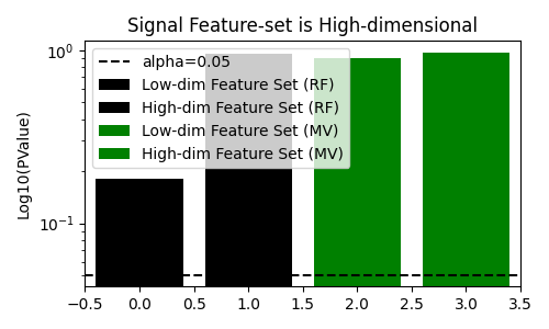
Estimated MI difference with first view (has dependency): -0.00010650682437673975 with Pvalue: 0.974025974025974
Estimated MI difference testing second view (does not have dependency): -9.142352901059247e-05 with Pvalue: 0.8931068931068931
Again, we compare to using a standard decision tree classifier as our base model.
covariate_index = np.arange(n_features_ends[0], dtype=int)
stat, pvalue = rf_est.test(X, y, covariate_index=covariate_index, metric="mi", n_repeats=n_repeats)

rf_results["low_dim_feature_stat"] = stat
rf_results["low_dim_feature_pvalue"] = pvalue
print("\n\nComparing with random forest.")
print(f"Estimated MI difference with first view (has dependency): {stat} with Pvalue: {pvalue}")

# we test for the second feature set, which is higher-dimensional
covariate_index = np.arange(n_features_ends[0], n_features_ends[1], dtype=int)
stat, pvalue = rf_est.test(
    X,
    y,
    covariate_index=covariate_index,
    metric="mi",
    n_repeats=n_repeats,
)
rf_results["high_dim_feature_stat"] = stat
rf_results["high_dim_feature_pvalue"] = pvalue
print(
    f"Estimated MI difference testing second view (does not have dependency): "
    f"{stat} with Pvalue: {pvalue}"
)

fig, ax = plt.subplots(figsize=(5, 3))

# plot pvalues
ax.bar(0, rf_results["low_dim_feature_pvalue"], label="Low-dim Feature Set (RF)", color="black")
ax.bar(1, rf_results["high_dim_feature_pvalue"], label="High-dim Feature Set (RF)", color="black")
ax.bar(2, mv_results["low_dim_feature_pvalue"], label="Low-dim Feature Set (MV)", color="green")
ax.bar(3, mv_results["high_dim_feature_pvalue"], label="High-dim Feature Set (MV)", color="green")
ax.axhline(0.05, color="k", linestyle="--", label="alpha=0.05")
ax.set(
    ylabel="Log10(PValue)",
    xlim=[-0.5, 3.5],
    yscale="log",
    title="Signal Feature-set is High-dimensional",
)
ax.legend()

fig.tight_layout()
plt.show()

Comparing with random forest.
Estimated MI difference with first view (has dependency): -0.0005592664624080035 with Pvalue: 0.18081918081918083
Estimated MI difference testing second view (does not have dependency): 0.0001352178572823215 with Pvalue: 0.9530469530469531
Discussion#
We see that when the null hypothesis is true, the multi-view decision tree does not reject the null hypothesis. In addition, it rejects the null hypothesis when there is a dependency between the target and the feature-set even when the feature-set is higher-dimensionality. This is in contrast to the standard decision tree, which fails to reject the null hypothesis when the feature-set with signal is higher-dimensional.
References#
Total running time of the script: (0 minutes 46.507 seconds)