Mutual Information for Genuine Hypothesis Testing (MIGHT) with Imbalanced Data

Here, we demonstrate how to do hypothesis testing on highly imbalanced data in terms of their feature-set dimensionalities. using mutual information as a test statistic. We use the framework of [1] to estimate pvalues efficiently.

Here, we simulate two feature sets, one of which is important for the target, but significantly smaller in dimensionality than the other feature set, which is unimportant for the target. We then use the MIGHT framework to test for the importance of each feature set. Instead of leveraging a normal honest random forest to estimate the posteriors, here we leverage a multi-view honest random forest, with knowledge of the multi-view structure of the X data.

For other examples of hypothesis testing, see the following:

• Mutual Information for Genuine Hypothesis Testing (MIGHT)

• Compute partial AUC using Mutual Information for Genuine Hypothesis Testing (MIGHT)

For more information on the multi-view decision-tree, see Analyze a multi-view dataset with a multi-view random forest.

import matplotlib.pyplot as plt
import numpy as np
from sklearn.datasets import make_blobs

from sktree import HonestForestClassifier
from sktree.stats import FeatureImportanceForestClassifier
from sktree.tree import DecisionTreeClassifier, MultiViewDecisionTreeClassifier

seed = 12345
rng = np.random.default_rng(seed)

Simulate data

We simulate the two feature sets, and the target variable. We then combine them into a single dataset to perform hypothesis testing.

seed = 12345
rng = np.random.default_rng(seed)


def make_multiview_classification(
    n_samples=100, n_features_1=10, n_features_2=1000, cluster_std=2.0, seed=None
):
    rng = np.random.default_rng(seed=seed)

    # Create a high-dimensional multiview dataset with a low-dimensional informative
    # subspace in one view of the dataset.
    X0_first, y0 = make_blobs(
        n_samples=n_samples,
        cluster_std=cluster_std,
        n_features=n_features_1 // 2,
        random_state=rng.integers(1, 10000),
        centers=1,
    )

    X1_first, y1 = make_blobs(
        n_samples=n_samples,
        cluster_std=cluster_std,
        n_features=n_features_1 // 2,
        random_state=rng.integers(1, 10000),
        centers=1,
    )

    # create the first views for y=0 and y=1
    X0_first = np.concatenate(
        (X0_first, rng.standard_normal(size=(n_samples, n_features_1 // 2))), axis=1
    )
    X1_first = np.concatenate(
        (X1_first, rng.standard_normal(size=(n_samples, n_features_1 // 2))), axis=1
    )
    y1[:] = 1

    # add the second view for y=0 and y=1, which is completely noise
    X0 = np.concatenate([X0_first, rng.standard_normal(size=(n_samples, n_features_2))], axis=1)
    X1 = np.concatenate([X1_first, rng.standard_normal(size=(n_samples, n_features_2))], axis=1)

    # combine the views and targets
    X = np.vstack((X0, X1))
    y = np.hstack((y0, y1)).T

    # add noise to the data
    X = X + rng.standard_normal(size=X.shape)

    return X, y


n_samples = 100
n_features = 10000
n_features_views = [10, n_features]

X, y = make_multiview_classification(
    n_samples=n_samples,
    n_features_1=10,
    n_features_2=n_features,
    cluster_std=2.0,
    seed=seed,
)

Perform hypothesis testing using Mutual Information

Here, we use FeatureImportanceForestClassifier to perform the hypothesis test. The test statistic is computed by comparing the metric (i.e. mutual information) estimated between two forests. One forest is trained on the original dataset, and one forest is trained on a permuted dataset, where the rows of the covariate_index columns are shuffled randomly.

The null distribution is then estimated in an efficient manner using the framework of [1]. The sample evaluations of each forest (i.e. the posteriors) are sampled randomly n_repeats times to generate a null distribution. The pvalue is then computed as the proportion of samples in the null distribution that are less than the observed test statistic.

n_estimators = 200
max_features = "sqrt"
test_size = 0.2
n_repeats = 1000
n_jobs = -1

est = FeatureImportanceForestClassifier(
    estimator=HonestForestClassifier(
        n_estimators=n_estimators,
        max_features=max_features,
        tree_estimator=MultiViewDecisionTreeClassifier(feature_set_ends=n_features_views),
        random_state=seed,
        honest_fraction=0.5,
        n_jobs=n_jobs,
    ),
    random_state=seed,
    test_size=test_size,
    permute_per_tree=False,
    sample_dataset_per_tree=False,
)

mv_results = dict()

print(
    f"Permutation per tree: {est.permute_per_tree} and sampling dataset per tree: "
    f"{est.sample_dataset_per_tree}"
)
# we test for the first feature set, which is important and thus should return a pvalue < 0.05
stat, pvalue = est.test(
    X, y, covariate_index=np.arange(10, dtype=int), metric="mi", n_repeats=n_repeats
)
mv_results["important_feature_stat"] = stat
mv_results["important_feature_pvalue"] = pvalue
print(f"Estimated MI difference: {stat} with Pvalue: {pvalue}")

# we test for the second feature set, which is unimportant and thus should return a pvalue > 0.05
stat, pvalue = est.test(
    X,
    y,
    covariate_index=np.arange(10, n_features, dtype=int),
    metric="mi",
    n_repeats=n_repeats,
)
mv_results["unimportant_feature_stat"] = stat
mv_results["unimportant_feature_pvalue"] = pvalue
print(f"Estimated MI difference: {stat} with Pvalue: {pvalue}")

Permutation per tree: False and sampling dataset per tree: False
Estimated MI difference: -0.6702887199082874 with Pvalue: 0.000999000999000999
Estimated MI difference: 0.0 with Pvalue: 0.5274725274725275

Let’s investigate what happens when we do not use a multi-view decision tree. All other parameters are kept the same.

est = FeatureImportanceForestClassifier(
    estimator=HonestForestClassifier(
        n_estimators=n_estimators,
        max_features=max_features,
        tree_estimator=DecisionTreeClassifier(),
        random_state=seed,
        honest_fraction=0.5,
        n_jobs=n_jobs,
    ),
    random_state=seed,
    test_size=test_size,
    permute_per_tree=False,
    sample_dataset_per_tree=False,
)

rf_results = dict()

# we test for the first feature set, which is important and thus should return a pvalue < 0.05
stat, pvalue = est.test(
    X, y, covariate_index=np.arange(10, dtype=int), metric="mi", n_repeats=n_repeats
)
rf_results["important_feature_stat"] = stat
rf_results["important_feature_pvalue"] = pvalue
print(f"Estimated MI difference using regular decision-trees: {stat} with Pvalue: {pvalue}")

# we test for the second feature set, which is unimportant and thus should return a pvalue > 0.05
stat, pvalue = est.test(
    X,
    y,
    covariate_index=np.arange(10, n_features, dtype=int),
    metric="mi",
    n_repeats=n_repeats,
)
rf_results["unimportant_feature_stat"] = stat
rf_results["unimportant_feature_pvalue"] = pvalue
print(f"Estimated MI difference using regular decision-trees: {stat} with Pvalue: {pvalue}")

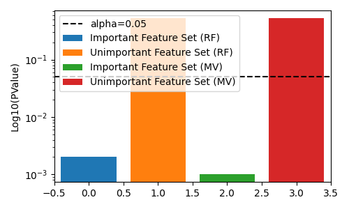
fig, ax = plt.subplots(figsize=(5, 3))

# plot pvalues
ax.bar(0, rf_results["important_feature_pvalue"], label="Important Feature Set (RF)")
ax.bar(1, rf_results["unimportant_feature_pvalue"], label="Unimportant Feature Set (RF)")
ax.bar(2, mv_results["important_feature_pvalue"], label="Important Feature Set (MV)")
ax.bar(3, mv_results["unimportant_feature_pvalue"], label="Unimportant Feature Set (MV)")
ax.axhline(0.05, color="k", linestyle="--", label="alpha=0.05")
ax.set(ylabel="Log10(PValue)", xlim=[-0.5, 3.5], yscale="log")
ax.legend()

fig.tight_layout()
plt.show()

Estimated MI difference using regular decision-trees: -0.005027243632117484 with Pvalue: 0.001998001998001998
Estimated MI difference using regular decision-trees: -0.00012290048360397154 with Pvalue: 0.5254745254745254

Discussion

We see that the multi-view decision tree is able to detect the important feature set, while the regular decision tree is not. This is because the regular decision tree is not aware of the multi-view structure of the data, and thus is challenged by the imbalanced dimensionality of the feature sets. I.e. it rarely splits on the first low-dimensional feature set, and thus is unable to detect its importance.

Note both approaches still fail to reject the null hypothesis (for alpha of 0.05) when testing the unimportant feature set. The difference in the two approaches show the statistical power of the multi-view decision tree is higher than the regular decision tree in this simulation.

References

[1] (1,2)

Tim Coleman, Wei Peng, and Lucas Mentch. Scalable and efficient hypothesis testing with random forests. The Journal of Machine Learning Research, 23(1):7679–7713, 2022.