1. Supervised Decision Trees

Supervised decision tree models are models where there is a ground-truth label, typically denoted y that is associated with each sample of data. In scikit-learn, the axis-aligned decision tree model is implemented and described. We extend those models beyond the axis-aligned tree model and describe their use-cases here.

1.1. Oblique Trees

Similar to DTs, Oblique Trees (OTs) are a non-parametric supervised learning method used for :ref: classification and :ref: regression. It was originally described as Forest-RC in Breiman’s landmark paper on Random Forests [RF]. Breiman found that combining data features empirically outperforms DTs on a variety of data sets.

The algorithm implemented in scikit-learn differs from Forest-RC in that it allows the user to specify the number of variables to combine to consider as a split, \(\lambda\). If \(\lambda\) is set to n_features, then it is equivalent to Forest-RC. \(\lambda\) presents a tradeoff between considering dense combinations of features vs sparse combinations of features.

1.1.1. Differences compared to decision trees

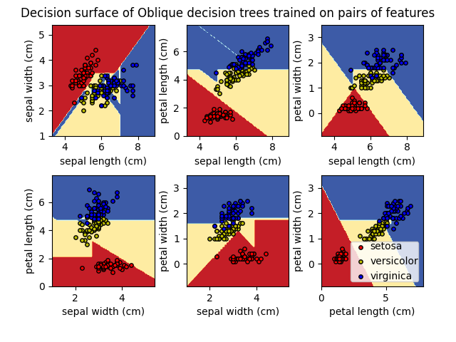
Compared to DTs, OTs differ in how they compute a candidate split. DTs split along the passed in data columns in an axis-aligned fashion, whereas OTs split along oblique curves. Using the Iris dataset, we can similarly construct an OT as follows:

>>> from sklearn.datasets import load_iris
>>> from sktree import tree
>>> iris = load_iris()
>>> X, y = iris.data, iris.target
>>> clf = tree.ObliqueDecisionTreeClassifier()
>>> clf = clf.fit(X, y)

Another major difference to DTs is that OTs can by definition sample more candidate splits. The parameter max_features controls how many splits to sample at each node. For DTs “max_features” is constrained to be at most “n_features” by default, whereas OTs can sample possibly up to \(2^{n_{features}}\) candidate splits because they are combining features.

1.1.2. Mathematical formulation

Given training vectors \(x_i \in R^n\), i=1,…, l and a label vector \(y \in R^l\), an oblique decision tree recursively partitions the feature space such that the samples with the same labels or similar target values are grouped together. Normal decision trees partition the feature space in an axis-aligned manner splitting along orthogonal axes based on the dimensions (columns) of \(x_i\). In oblique trees, nodes sample a random projection vector, \(a_i \in R^n\), where the inner-product of \(\langle a_i, x_i \rangle\) is a candidate split value. The entries of \(a_i\) have values +/- 1 with probability \(\lambda / n\) with the rest being 0s.

Let the data at node \(m\) be represented by \(Q_m\) with \(n_m\) samples. For each candidate split \(\theta = (a_i, t_m)\) consisting of a (possibly sparse) vector \(a_i\) and threshold \(t_m\), partition the data into \(Q_m^{left}(\theta)\) and \(Q_m^{right}(\theta)\) subsets

\[ \begin{align}\begin{aligned}Q_m^{left}(\theta) = \{(x, y) | a_i^T x_j \leq t_m\}\\Q_m^{right}(\theta) = Q_m \setminus Q_m^{left}(\theta)\end{aligned}\end{align} \]

Note that this formulation is a generalization of decision trees, where \(a_i = e_i\), a standard basis vector with a “1” at index “i” and “0” elsewhere.

The quality of a candidate split of node \(m\) is then computed using an impurity function or loss function \(H()\), in the same exact manner as decision trees.

1.1.3. Classification, regression and multi-output problems

OTs can be used for both classification and regression, and can handle multi-output problems in the same manner as DTs.

1.1.4. Complexity

The run time cost to construct an OT will be similar to that of a DT, with the added complexity of a (possibly sparse) matrix multiplication to combine random data columns into candidate split values. The cost at each node is \(O(n_{features}n_{samples}\log(n_{samples}) + n_{features}n_{samples}max\_features \lambda)\) where the additional \(n_{features}n_{samples}max\_features \lambda\) term comes from the (possibly sparse) matrix multiplication controlled by both the number of candidate splits to generate (“max_features”) and the sparsity of the projection matrix that combines the data features (”\(\lambda\)”).

Another consideration is space-complexity.

Space-complexity and storing the OT pickled on disc is also a consideration. OTs at every node need to store an additional vector of feature indices and vector of feature weights that are used together to form the candidate splits.

1.1.5. Tips on practical use

Similar to DTs, the intuition for most parameters are the same. Therefore refer to tips for using decision trees for information on standard tree parameters. Specific parameters, such as max_features and feature_combinations are different or special to OTs.

• As specified earlier, max_features is not constrained to n_features as it is in DTs. Setting max_features higher requires more computation time because the algorithm needs to sample more candidate splits at every node. However, it also possibly lets the user to sample more informative splits, thereby improving the model fit. This presents a tradeoff between runtime resources and improvements to the model. In practice, we found that sampling more splits, say up to max_features=n_features**2, is desirable if one is willing to spend the computational resources.

• feature_combinations is the \(\lambda\) term presented in the complexity analysis, which specifies how sparse our combination of features is. If feature_combinations=n_features, then OT is the Forest-RC version. However, in practice, feature_combinations can be set much lower, therefore improving runtime and storage complexity.

Finally, when asking the question of when to use OTs vs DTs, scikit-learn recommends always trying both model using some type of cross-validation procedure and hyperparameter optimization (e.g. GridSearchCV). If one has prior knowledge about how the data is distributed along its features, such as data being axis-aligned, then one might use a DT. Other considerations are runtime and space complexity.

1.1.6. Limitations compared to decision trees

• There currently does not exist support for pruning OTs, such as with the minimal cost-complexity pruning algorithm.

• Moreover, OTs do not have built-in support for missing data, so the recommendation by scikit-learn is for users to first impute, or drop their missing data if they would like to use OTs.

• Currently, OTs also does not support sparse inputs for data matrices and labels.

References:

[RF]

L. Breiman. Random Forests. Machine Learning 45, 5–32 (2001). https://doi.org/10.1023/A:1010933404324.

• https://en.wikipedia.org/wiki/Decision_tree_learning

• https://en.wikipedia.org/wiki/Predictive_analytics

• J.R. Quinlan. C4. 5: programs for machine learning. Morgan Kaufmann, 1993.

• T. Hastie, R. Tibshirani and J. Friedman. Elements of Statistical Learning, Springer, 2009.

1.2. Honest Trees

Honesty is a property of decision trees where the data used to determine splitting is independent of the data used to estimate the prediction at each leaf. This is in contrast to standard decision where the data used to determine splitting is also used to estimate the prediction at each leaf.

Honesty is a desirable property because it prevents overfitting. In particular, it prevents the tree from overfitting to the training data. This is because the data used to determine splitting is independent of the data used to estimate the prediction at each leaf.

There are two methods for constructing an honest tree: 1. subsampling and 2. propensity trees. The first method, subsampling, is the most common method for constructing honest trees and only requires (X, y) pairs of data. The second method, propensity trees, requires (X, y, T) triplets where the tree is split first using (X, T), where T is the treatment variable, and then the prediction at each leaf is estimated using (X, y).

Honesty results in calibrated confidence intervals, but sacrifices sample size to do so. Thus subsampled honest trees have higher MSE, but are better calibrated. See :