Comparing a-Priori SBM Fitting with Different Groupings¶

It is often desirable to create models of data so we can generate new samples, learn something about the data’s structure, or for use in some larger analysis. SBM models define different connection probabilities for different communities in a graph.

Here we enforce a community structure a-priori based a some connectome attributes or combinations thereof, and fit an SBM. In this case, the connection probability between two blocks is simply the total number of observed connections between them, divided by the total number of possible connections between them.

We fit these SBMs using different attributes or combinations of attributes from the connectome, and then compute the BIC (Bayesian Information Criterion) for each model. This gives us an idea of which attributes best explain the topological structure of the connectome.

For consistency, we use the attributes hemisphere (the side of the brain a neuron is on), cell_type (the high-level classification of a neuron as interneuron, sensory, or motor) and their combination as groups for fitting. The analysis is only preformed on the Ciona Intestinalis Connectome, two C. Elegans Worm Wiring Connectomes, and the 8 C. Elegans Developmental Connectomes, because only these have both those attributes defined.

Note that the code to do the actual SBM fitting is located in analysis/apriori_sbm_code.py

import os
import sys
import matplotlib.pyplot as plt
sys.path.append("../")
import pandas as pd
from graph import GraphIO
from analysis.apriori_sbm_code import fit_apriori_sbm
import seaborn as sns
import numpy as np

Ciona Intestinalis¶

We’ll start with the single Ciona Connectome. First we load the data:

path = '../json_connectomes/ciona.json'
ciona_connectome, _, _, _ = GraphIO.load(path)

Now we’ll fit an SBM for each grouping

# In Ciona, Hemisphere is called side and cell_type is called annotation
groups = [['Side'], ['Annotation'], ['Side', 'Annotation']]
rows = {'Ciona Intestinalis': {}}
for group in groups:
    rows['Ciona Intestinalis'][str(group)] = fit_apriori_sbm(ciona_connectome, group, plot_sbms=False)
ciona_results = pd.DataFrame.from_dict({(i,j): rows[i][j]
                           for i in rows.keys()
                           for j in rows[i].keys()},
                       orient='index')
ciona_results.head()

		bic	likelihood	n_params	estimator
Ciona Intestinalis	['Side']	-23033.922165	-10863.237119	121	SBMEstimator()
	['Annotation']	-22820.202349	-11323.658336	16	SBMEstimator()
	['Side', 'Annotation']	-26206.331665	-10245.149497	529	SBMEstimator()

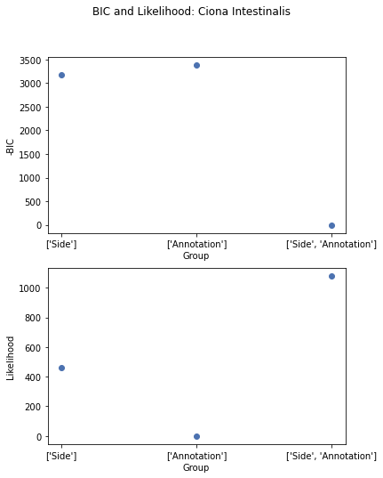
Great, now lets plot -BIC for different groupings. The lowest -BIC is set to 0, since the scale doesn’t really matter here.

colors = sns.color_palette("deep")[0]
fig, ax = plt.subplots(2, 1)
out_index = ciona_results.index.levels[0]
for i, key in enumerate(out_index):
    data = ciona_results.loc[key]
    bic_data = data['bic'].to_numpy()
    norm_bic = bic_data - np.min(bic_data)
    like_data = data['likelihood'].to_numpy()
    norm_like = like_data - np.min(like_data)
    _ = ax[0].scatter(data['bic'].index,
                  norm_bic,
                  label=key,
                  color=np.array(colors))
    _ = ax[1].scatter(data['likelihood'].index,
                  norm_like,
                  label=key,
                  color=np.array(colors))
    _ = ax[0].set(xlabel='Group', ylabel='-BIC')
    _ = ax[1].set(xlabel='Group', ylabel='Likelihood')
_ = fig.suptitle('BIC and Likelihood: Ciona Intestinalis')
_ = fig.set_size_inches(6, 8)

It appears annotation has the best BIC but the worst likelihood. This could be because annotation has much fewer parameters than the other groupings. (For Ciona ‘Side’ is broken into 11 groupings instead of just ‘Left’ and ‘Right’). Therefore, based on the BIC, annotation explains the structure better, and the other groupings are likely fitting noise.

C. Elegans Developmental Conectomes (Witviliet)¶

We will preform this analysis for all 8 developmental stages at once.

# load some elegans Witvliet data
base = '../json_connectomes/witvilet/'
graph_files = sorted(os.listdir(base))
wit_connectomes = []
for f in graph_files:
    # These contain multiple synapse types, and thus can have multiedges and need to be flattened.
    # Alternatively, we could preform the analysis separately for each synapse type
    wit_connectomes.append(GraphIO.flatten_multigraph(GraphIO.load(os.path.join(base, f))[0]))

Now we will fit sbms for each grouping for each connectome.

groups = [["hemisphere"], ["cell_type0"], ["hemisphere", "cell_type0"]]
rows = {}
ages = []
for i in range(len(wit_connectomes)):
    age = wit_connectomes[i].graph['age']
    ages.append(age)
    g_row = {}
    for group in groups:
        g_row[str(group)] = fit_apriori_sbm(wit_connectomes[i], group, plot_sbms=False)
    rows['Witvliet ' + str(age) + ' hours'] = g_row
wit_results = pd.DataFrame.from_dict({(i,j): rows[i][j]
                           for i in rows.keys()
                           for j in rows[i].keys()},
                       orient='index')
ages = np.array(ages)
wit_results.head(24)

		bic	likelihood	n_params	estimator
Witvliet 0 hours	['hemisphere']	-8016.577339	-3961.208692	9	SBMEstimator()
	['cell_type0']	-7651.218552	-3694.831560	25	SBMEstimator()
	['hemisphere', 'cell_type0']	-8917.613900	-3574.749594	169	SBMEstimator()
Witvliet 5 hours	['hemisphere']	-9913.659242	-4909.418897	9	SBMEstimator()
	['cell_type0']	-9401.135504	-4510.924858	36	SBMEstimator()
	['hemisphere', 'cell_type0']	-10818.117288	-4376.558445	196	SBMEstimator()
Witvliet 8 hours	['hemisphere']	-10035.203502	-4970.007348	9	SBMEstimator()
	['cell_type0']	-9387.116384	-4561.351516	25	SBMEstimator()
	['hemisphere', 'cell_type0']	-10628.877074	-4420.721409	169	SBMEstimator()
Witvliet 16 hours	['hemisphere']	-11716.860426	-5810.567133	9	SBMEstimator()
	['cell_type0']	-10907.811713	-5320.952857	25	SBMEstimator()
	['hemisphere', 'cell_type0']	-12142.430570	-5172.453006	169	SBMEstimator()
Witvliet 23 hours	['hemisphere']	-14771.539210	-7337.602882	9	SBMEstimator()
	['cell_type0']	-13806.911934	-6710.789074	36	SBMEstimator()
	['hemisphere', 'cell_type0']	-15164.255483	-6533.163547	196	SBMEstimator()
Witvliet 27 hours	['hemisphere']	-14586.909618	-7245.077303	9	SBMEstimator()
	['cell_type0']	-13437.319264	-6584.277672	25	SBMEstimator()
	['hemisphere', 'cell_type0']	-14596.318736	-6389.737317	169	SBMEstimator()
Witvliet 45 hours	['hemisphere']	-19049.862125	-9476.429417	9	SBMEstimator()
	['cell_type0']	-17546.406610	-8579.196723	36	SBMEstimator()
	['hemisphere', 'cell_type0']	-19108.022424	-8341.470073	225	SBMEstimator()

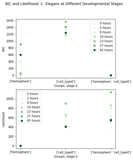
Let’s plot -BIC for different groupings. Again the lowest -BIC for each developmental stage is set to 0, allowing for easy comparison.

fig, ax = plt.subplots(2)
out_index = wit_results.index.levels[0]
cm = plt.cm.get_cmap('Greens')
colors = cm(ages/max(ages))
for i, key in enumerate(out_index):
    data = wit_results.loc[key]
    bic_data = data['bic'].to_numpy()
    norm_bic = bic_data - np.min(bic_data)
    like_data = data['likelihood'].to_numpy()
    norm_like = like_data - np.min(like_data)
    _ = ax[0].scatter(data['bic'].index,
                     norm_bic,
                     label=str(ages[i]) + ' hours',
                     color=np.array(colors)[i])
    _ = ax[1].scatter(data['likelihood'].index,
                     norm_like,
                     label=str(ages[i]) + ' hours',
                     color=np.array(colors)[i])
    _ = ax[0].set(xlabel='Groups, stage ' + str(i), ylabel='-BIC')
    _ = ax[1].set(xlabel='Groups, stage ' + str(i), ylabel='Likelihood')
_ = fig.suptitle('BIC and Likelihood: C. Elegans at Different Developmental Stages')
_ = fig.set_size_inches(6, 8)
_ = ax[0].legend(loc='best')
_ = ax[1].legend(loc='best')

Once again, we find that cell type explains the topology the best. This is still not entirely surprising, since the connectivity of interneurons should be very different than that of sensory or motor neurons

C. Elegans Male and Hermaphrodite Conectomes (Worm Wiring)¶

# load chemical synapse connectome files
path_h = '../json_connectomes/worm_wiring/connectome/Hermaphrodite/0.json'
path_m = '../json_connectomes/worm_wiring/connectome/Male/0.json'
ww_connectomes = []
ww_connectomes.append(GraphIO.load(path_h)[0])
ww_connectomes.append(GraphIO.load(path_m)[0])

groups = [["hemisphere"], ["cell_type0"], ["hemisphere", "cell_type0"]]
types = ['Hermaphrodite', 'Male']
rows = {}
for i in range(len(ww_connectomes)):
    g_row = {}
    for group in groups:
        g_row[str(group)] = fit_apriori_sbm(ww_connectomes[i], group, plot_sbms=False)
    rows['C. Elegans ' + types[i]] = g_row
ww_results = pd.DataFrame.from_dict({(i,j): rows[i][j]
                           for i in rows.keys()
                           for j in rows[i].keys()},
                       orient='index')
ww_results.head(6)

		bic	likelihood	n_params	estimator
C. Elegans Hermaphrodite	['hemisphere']	-45484.654884	-22687.264567	9	SBMEstimator()
	['cell_type0']	-37783.419558	-18500.151558	64	SBMEstimator()
	['hemisphere', 'cell_type0']	-41098.822390	-17588.252151	484	SBMEstimator()
C. Elegans Male	['hemisphere']	-53425.404138	-26655.512739	9	SBMEstimator()
	['cell_type0']	-43612.375238	-21399.507936	64	SBMEstimator()
	['hemisphere', 'cell_type0']	-47806.496439	-20541.786468	529	SBMEstimator()

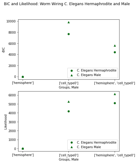
One last time, we’ll plot -BIC and Likelihood, the lowest -BIC is again set to 0.

fig, ax = plt.subplots(2)
out_index = ww_results.index.levels[0]
colors = sns.color_palette("dark")[2]
for i, key in enumerate(out_index):
    data = ww_results.loc[key]
    bic_data = data['bic'].to_numpy()
    norm_bic = bic_data - np.min(bic_data)
    like_data = data['likelihood'].to_numpy()
    norm_like = like_data - np.min(like_data)
    if 'Male' in key:
        shape = '^'
    else:
        shape = 'o'
    _ = ax[0].scatter(data['bic'].index,
                     norm_bic,
                     label=key,
                     color=np.array(colors),
                     marker=shape,)
    _ = ax[1].scatter(data['likelihood'].index,
                     norm_like,
                     label=key,
                     color=np.array(colors),
                     marker=shape,)
    _ = ax[0].set(xlabel='Groups, ' + types[i], ylabel='-BIC')
    _ = ax[1].set(xlabel='Groups, ' + types[i], ylabel='Likelihood')
_ = ax[0].legend(loc='best')
_ = ax[1].legend(loc='best')
_ = fig.suptitle('BIC and Likelihood: Worm Wiring C. Elegans Hermaphrodite and Male')
_ = fig.set_size_inches(6, 8)

For a third time, cell type groupings get the best BIC. This makes sense since this is the same species as the developmental data

Connectocross

Comparing a-Priori SBM Fitting with Different Groupings¶

Ciona Intestinalis¶

C. Elegans Developmental Conectomes (Witviliet)¶

C. Elegans Male and Hermaphrodite Conectomes (Worm Wiring)¶